Bayesian Computation with R

4.2 パラメータが二つとも未知の正規データ
> data(marathontimes)
> attach(marathontimes)

> d = mycontour(normchi2post, c(220, 330, 500, 9000), time,
+ xlab=”mean”,ylab=”variance”)
> S = sum((time – mean(time))^2)
> n = length(time)
> sigma2 = S/rchisq(1000, n – 1)
> mu = rnorm(1000, mean = mean(time), sd = sqrt(sigma2)/sqrt(n))
> points(mu, sigma2)

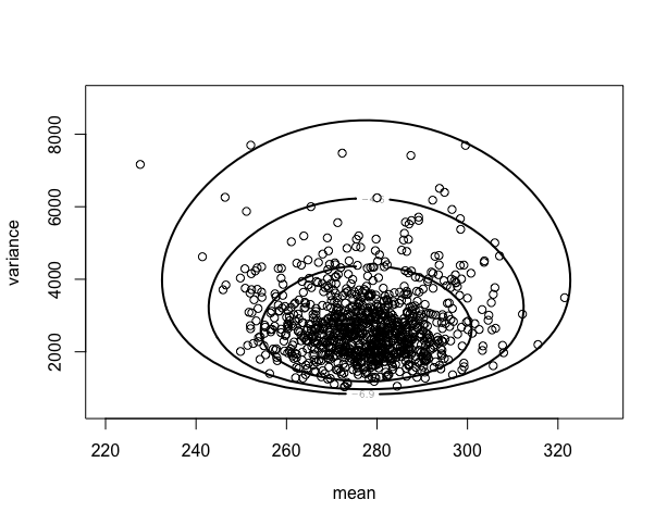
> quantile(mu, c(0.025, 0.975))
2.5% 97.5%
253.7060 300.0964
>
> quantile(sqrt(sigma2), c(0.025, 0.975))
2.5% 97.5%
37.04298 71.47564

4.3 多項モデル
> alpha = c(728, 584, 138)
> theta = rdirichlet(1000, alpha)
> hist(theta[, 1] – theta[, 2], main=””)

> data(election.2008)
> attach(election.2008)
>
> prob.Obama=function(j)
+ {
+ p=rdirichlet(5000,
+ 500*c(M.pct[j],O.pct[j],100-M.pct[j]-O.pct[j])/100+1)
+ mean(p[,2]>p[,1])
+ }
>
> Obama.win.probs=sapply(1:51,prob.Obama)

> sim.election=function()
+ {
+ winner=rbinom(51,1,Obama.win.probs)
+ sum(EV*winner)
+ }
>
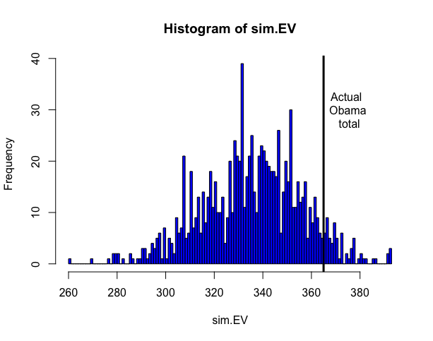
> sim.EV=replicate(1000,sim.election())

> hist(sim.EV,min(sim.EV):max(sim.EV),col=”blue”)
> abline(v=365,lwd=3) # Obama received 365 votes
> text(375,30,”Actual \n Obama \n total”)

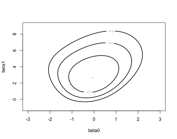
4.4 生物検定実験
> x = c(-0.86, -0.3, -0.05, 0.73)
> n = c(5, 5, 5, 5)
> y = c(0, 1, 3, 5)
> data = cbind(x, n, y)

> glmdata = cbind(y, n – y)
> results = glm(glmdata ~ x, family = binomial)
> summary(results)

Call:
glm(formula = glmdata ~ x, family = binomial)

Deviance Residuals:
1 2 3 4
-0.17236 0.08133 -0.05869 0.12237

Coefficients:
Estimate Std. Error z value Pr(>|z|)
(Intercept) 0.8466 1.0191 0.831 0.406
x 7.7488 4.8728 1.590 0.112

(Dispersion parameter for binomial family taken to be 1)

Null deviance: 15.791412 on 3 degrees of freedom
Residual deviance: 0.054742 on 2 degrees of freedom
AIC: 7.9648

Number of Fisher Scoring iterations: 7

> beta.select(list(p=.5,x=.2),list(p=.9,x=.5))
[1] 1.12 3.56
> beta.select(list(p=.5,x=.8),list(p=.9,x=.98))
[1] 2.10 0.74

> prior=rbind(c(-0.7, 4.68, 1.12),
+ c(0.6, 2.10, 0.74))
> data.new=rbind(data, prior)

> mycontour(logisticpost,c(-3,3,-1,9),data.new,
+ xlab=”beta0″, ylab=”beta1″)

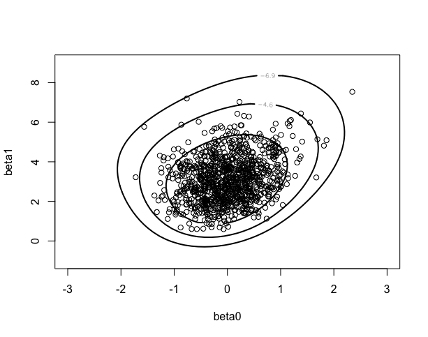
> s=simcontour(logisticpost,c(-2,3,-1,11),data.new,1000)
> points(s)

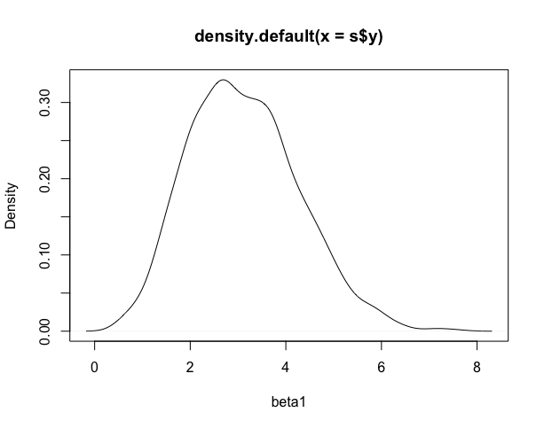
> plot(density(s$y),xlab=”beta1″)

> theta=-s$x/s$y
>
> hist(theta,xlab=”LD-50″,breaks=20)

> quantile(theta,c(.025,.975))
2.5% 97.5%
-0.3314614 0.5195462

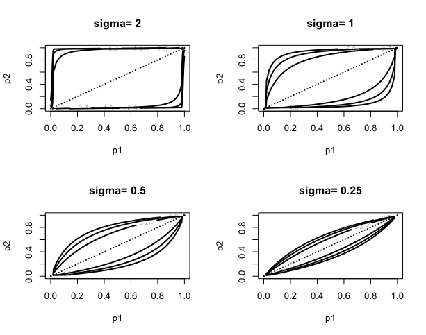
4.5 二つの割合を比較する
> sigma=c(2,1,.5,.25)
> plo=.0001;phi=.9999
> par(mfrow=c(2,2))
> for (i in 1:4)
+ mycontour(howardprior,c(plo,phi,plo,phi),c(1,1,1,1,sigma[i]),
+ main=paste(“sigma=”,as.character(sigma[i])),
+ xlab=”p1″,ylab=”p2″)
>
>

> sigma=c(2,1,.5,.25)
> if (.Platform$OS.type == “unix”) x11() else windows()
> par(mfrow=c(2,2))
> for (i in 1:4)
+ {
+ mycontour(howardprior,c(plo,phi,plo,phi),
+ c(1+3,1+15,1+7,1+5,sigma[i]),
+ main=paste(“sigma=”,as.character(sigma[i])),
+ xlab=”p1″,ylab=”p2″)
+ lines(c(0,1),c(0,1))

> s=simcontour(howardprior,c(plo,phi,plo,phi),
+ c(1+3,1+15,1+7,1+5,2),1000)
> sum(s$x>s$y)/1000
[1] 0.018