機械学習の学習１Pythonによる機械学習入門（オーム社）から
ーーーーーーーーーーーーーーーーーーーーーーーーーーーーーーーーーーーーーーーーーー
準備段階Graphvisのインストール
ーーーーーーーーーーーーーーーーーーーーーーーーーーーーーーーーーーーーーーーーーー
http://www.graphviz.org
まずは、dotファイルを画像化するためにgraphvizをMac OS X(Sierra)にインストールした。
http://macappstore.org/graphviz-2/　を参考に
Terminalから、基本は
$ brew install graphviz
なんだけど、悪戦苦闘した。
Format: “png” not recognized. Use one of:等のエラーで動かない。
https://github.com/ContinuumIO/anaconda-issues/issues/485
を参考に、
% conda create -n graphviz python graphviz
% which dot
activate graphviz
でやっとコマンドラインから
$dot -T png graph.dot -o graph.pdf　等でpdfゃpngへdotファイルが変換可能となった。
ーーーーーーーーーーーーーーーーーーーーーーーーーーーーーーーーーーーーーーーーーー
Scikit-learnでClassification問題を学習する：手書きの数字を自動認識する分類器の作成
ーーーーーーーーーーーーーーーーーーーーーーーーーーーーーーーーーーーーーーーーーー
import matplotlib.pyplot as plt
from sklearn import datasets

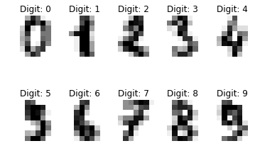
# 手書き数字データの読み込み
digits = datasets.load_digits()

# 画像を 2 行 5 列に表示
for label, img in zip(digits.target[:10], digits.images[:10]):
　　plt.subplot(2, 5, label + 1)
　　plt.axis(‘off’)
　　plt.imshow(img, cmap=plt.cm.gray_r, interpolation=’nearest’)
　　plt.title(‘Digit: {0}’.format(label))
plt.show()
ーーーーーーーーーーーーーーーーーーーーーーーーーーーーーーーーーーーーーーーーーー

ーーーーーーーーーーーーーーーーーーーーーーーーーーーーーーーーーーーーーーーーーー
3と8の画像を分類する。
ーーーーーーーーーーーーーーーーーーーーーーーーーーーーーーーーーーーーーーーーーー
import numpy as np
from sklearn import datasets

# 手書き数字データの読み込み
digits = datasets.load_digits()

# 3 と 8 のデータ位置を求める
flag_3_8 = (digits.target == 3) + (digits.target == 8)

# 3 と 8 のデータを取得
images = digits.images[flag_3_8]
labels = digits.target[flag_3_8]

# 3 と 8 の画像データを 1 次元化
images = images.reshape(images.shape[0], -1)

ーーーーーーーーーーーーーーーーーーーーーーーーーーーーーーーーーーーーーーーーーー
分類器を生成して学習を実施
ーーーーーーーーーーーーーーーーーーーーーーーーーーーーーーーーーーーーーーーーーー
from sklearn import tree

# 3 と 8 の画像データを 1 次元化
images = images.reshape(images.shape[0], -1)

# 分類器の生成
n_samples = len(flag_3_8[flag_3_8])
train_size = int(n_samples * 3 / 5)
classifier = tree.DecisionTreeClassifier()
classifier.fit(images[:train_size], labels[:train_size])
ーーーーーーーーーーーーーーーーーーーーーーーーーーーーーーーーーーーーーーーーーー
DecisionTreeClassifier(class_weight=None, criterion=’gini’, max_depth=None,
max_features=None, max_leaf_nodes=None,
min_impurity_decrease=0.0, min_impurity_split=None,
min_samples_leaf=1, min_samples_split=2,
min_weight_fraction_leaf=0.0, presort=False, random_state=None,
splitter=’best’)
ーーーーーーーーーーーーーーーーーーーーーーーーーーーーーーーーーーーーーーーーーー
分類器の性能を計算
ーーーーーーーーーーーーーーーーーーーーーーーーーーーーーーーーーーーーーーーーーー
from sklearn.metrics import accuracy_score, confusion_matrix
from sklearn.metrics import precision_score, recall_score, f1_score

from sklearn.metrics import accuracy_score, confusion_matrix
from sklearn.metrics import precision_score, recall_score, f1_score

# 分類器の性能の確認
expected = labels[train_size:]
predicted = classifier.predict(images[train_size:])

print(‘Accuracy:\n’, accuracy_score(expected, predicted))
print(‘Confusion matrix:\n’, confusion_matrix(expected, predicted))
print(‘Precision:\n’, precision_score(expected, predicted, pos_label=3))
print(‘Recall:\n’, recall_score(expected, predicted, pos_label=3))
print(‘F-measure:\n’, f1_score(expected, predicted, pos_label=3))
ーーーーーーーーーーーーーーーーーーーーーーーーーーーーーーーーーーーーーーーーーー
Accuracy:
0.881118881119
Confusion matrix:
[[60 15]
[ 2 66]]
Precision:
0.967741935484
Recall:
0.8
F-measure:
0.875912408759
ーーーーーーーーーーーーーーーーーーーーーーーーーーーーーーーーーーーーーーーーーー
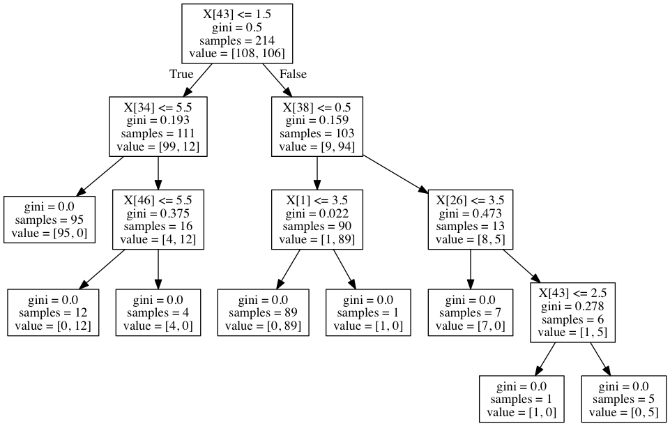
# 学習した結果をGraphvizが認識できる形式にして出力する
ーーーーーーーーーーーーーーーーーーーーーーーーーーーーーーーーーーーーーーーーーー
with open(‘graph_1.dot’, ‘w’) as f:
f = tree.export_graphviz(classifier, out_file=f)
ーーーーーーーーーーーーーーーーーーーーーーーーーーーーーーーーーーーーーーーーーー
コマンドラインから
$ dot -Tpng graph_1.dot -o graph_1.png
ーーーーーーーーーーーーーーーーーーーーーーーーーーーーーーーーーーーーーーーーーー

ーーーーーーーーーーーーーーーーーーーーーーーーーーーーーーーーーーーーーーーーーー
コードを弄ってみる１
ーーーーーーーーーーーーーーーーーーーーーーーーーーーーーーーーーーーーーーーーーー
import matplotlib.pyplot as plt
from sklearn import datasets

# 手書き数字データの読み込み
digits = datasets.load_digits()

# 画像を 2 行 5 列に表示
for label, img in zip(digits.target[10:20], digits.images[10:20]):
plt.subplot(1, 10, label + 1)
plt.axis(‘on’)
plt.imshow(img, cmap=plt.cm.gray_r, interpolation=’nearest’)
plt.title(‘Digit: {0}’.format(label))
plt.show()
ーーーーーーーーーーーーーーーーーーーーーーーーーーーーーーーーーーーーーーーーーー

ーーーーーーーーーーーーーーーーーーーーーーーーーーーーーーーーーーーーーーーーーー
from sklearn import tree

# 3 と 8 の画像データを 1 次元化
images = images.reshape(images.shape[0], -1)

# 分類器の生成
n_samples = len(flag_3_8[flag_3_8])
train_size = int(n_samples * 2 / 5)
classifier = tree.DecisionTreeClassifier(max_depth=5)
classifier.fit(images[:train_size], labels[:train_size])

from sklearn.metrics import accuracy_score, confusion_matrix
from sklearn.metrics import precision_score, recall_score, f1_score
ーーーーーーーーーーーーーーーーーーーーーーーーーーーーーーーーーーーーーーーーーー
# 分類器の性能の確認
expected = labels[train_size:]
predicted = classifier.predict(images[train_size:])

print(‘Accuracy:\n’, accuracy_score(expected, predicted))
print(‘Confusion matrix:\n’, confusion_matrix(expected, predicted))
print(‘Precision:\n’, precision_score(expected, predicted, pos_label=3))
print(‘Recall:\n’, recall_score(expected, predicted, pos_label=3))
print(‘F-measure:\n’, f1_score(expected, predicted, pos_label=3))
ーーーーーーーーーーーーーーーーーーーーーーーーーーーーーーーーーーーーーーーーーー
Accuracy:
0.888372093023
Confusion matrix:
[[96 15]
[ 9 95]]
Precision:
0.914285714286
Recall:
0.864864864865
F-measure:
0.888888888889
ーーーーーーーーーーーーーーーーーーーーーーーーーーーーーーーーーーーーーーーーーー
# 学習した結果をGraphvizが認識できる形式にして出力する
with open(‘graph_2.dot’, ‘w’) as f:
f = tree.export_graphviz(classifier, out_file=f)
ーーーーーーーーーーーーーーーーーーーーーーーーーーーーーーーーーーーーーーーーーー