前日の続き: 深層学習
——————————————————–
digitsのデータ構造はどうなっているのか?
——————————————————–
In: digits
Out: {‘DESCR’: “Optical Recognition of Handwritten Digits Data Set\n===================================================\n\nNotes\n—–\nData Set Characteristics:\n :Number of Instances: 5620\n :Number of Attributes: 64\n :Attribute Information: 8×8 image of integer pixels in the range 0..16.\n :Missing Attribute Values: None\n :Creator: E. Alpaydin (alpaydin ‘@’ boun.edu.tr)\n :Date: July; 1998\n\nThis is a copy of the test set of the UCI ML hand-written digits datasets\nhttp://archive.ics.uci.edu/ml/datasets/Optical+Recognition+of+Handwritten+Digits\n\nThe data set contains images of hand-written digits: 10 classes where\neach class refers to a digit.\n\nPreprocessing programs made available by NIST were used to extract\nnormalized bitmaps of handwritten digits from a preprinted form. From a\ntotal of 43 people, 30 contributed to the training set and different 13\nto the test set. 32×32 bitmaps are divided into nonoverlapping blocks of\n4x4 and the number of on pixels are counted in each block. This generates\nan input matrix of 8×8 where each element is an integer in the range\n0..16. This reduces dimensionality and gives invariance to small\ndistortions.\n\nFor info on NIST preprocessing routines, see M. D. Garris, J. L. Blue, G.\nT. Candela, D. L. Dimmick, J. Geist, P. J. Grother, S. A. Janet, and C.\nL. Wilson, NIST Form-Based Handprint Recognition System, NISTIR 5469,\n1994.\n\nReferences\n———-\n – C. Kaynak (1995) Methods of Combining Multiple Classifiers and Their\n Applications to Handwritten Digit Recognition, MSc Thesis, Institute of\n Graduate Studies in Science and Engineering, Bogazici University.\n – E. Alpaydin, C. Kaynak (1998) Cascading Classifiers, Kybernetika.\n – Ken Tang and Ponnuthurai N. Suganthan and Xi Yao and A. Kai Qin.\n Linear dimensionalityreduction using relevance weighted LDA. School of\n Electrical and Electronic Engineering Nanyang Technological University.\n 2005.\n – Claudio Gentile. A New Approximate Maximal Margin Classification\n Algorithm. NIPS. 2000.\n”,
‘data’: array([[ 0., 0., 5., …, 0., 0., 0.],
[ 0., 0., 0., …, 10., 0., 0.],
[ 0., 0., 0., …, 16., 9., 0.],
…,
[ 0., 0., 1., …, 6., 0., 0.],
[ 0., 0., 2., …, 12., 0., 0.],
[ 0., 0., 10., …, 12., 1., 0.]]),
‘images’: array([[[ 0., 0., 5., …, 1., 0., 0.],
[ 0., 0., 13., …, 15., 5., 0.],
[ 0., 3., 15., …, 11., 8., 0.],
…,
[ 0., 4., 11., …, 12., 7., 0.],
[ 0., 2., 14., …, 12., 0., 0.],
[ 0., 0., 6., …, 0., 0., 0.]],
[[ 0., 0., 0., …, 5., 0., 0.],
[ 0., 0., 0., …, 9., 0., 0.],
[ 0., 0., 3., …, 6., 0., 0.],
…,
[ 0., 0., 1., …, 6., 0., 0.],
[ 0., 0., 1., …, 6., 0., 0.],
[ 0., 0., 0., …, 10., 0., 0.]],
[[ 0., 0., 0., …, 12., 0., 0.],
[ 0., 0., 3., …, 14., 0., 0.],
[ 0., 0., 8., …, 16., 0., 0.],
…,
[ 0., 9., 16., …, 0., 0., 0.],
[ 0., 3., 13., …, 11., 5., 0.],
[ 0., 0., 0., …, 16., 9., 0.]],
…,
[[ 0., 0., 1., …, 1., 0., 0.],
[ 0., 0., 13., …, 2., 1., 0.],
[ 0., 0., 16., …, 16., 5., 0.],
…,
[ 0., 0., 16., …, 15., 0., 0.],
[ 0., 0., 15., …, 16., 0., 0.],
[ 0., 0., 2., …, 6., 0., 0.]],
[[ 0., 0., 2., …, 0., 0., 0.],
[ 0., 0., 14., …, 15., 1., 0.],
[ 0., 4., 16., …, 16., 7., 0.],
…,
[ 0., 0., 0., …, 16., 2., 0.],
[ 0., 0., 4., …, 16., 2., 0.],
[ 0., 0., 5., …, 12., 0., 0.]],
[[ 0., 0., 10., …, 1., 0., 0.],
[ 0., 2., 16., …, 1., 0., 0.],
[ 0., 0., 15., …, 15., 0., 0.],
…,
[ 0., 4., 16., …, 16., 6., 0.],
[ 0., 8., 16., …, 16., 8., 0.],
[ 0., 1., 8., …, 12., 1., 0.]]]),
‘target’: array([0, 1, 2, …, 8, 9, 8]),
‘target_names’: array([0, 1, 2, 3, 4, 5, 6, 7, 8, 9])}
——————————————————–
つまり、DESCR(デスクリプション)に続いて、
1) ‘data’:array
2) ‘images’:array
3) ‘target’:array
4) ‘target_names’:array
と4つの配列で構成されていることが解った。
——————————————————–
始めのデータはどうなっているのか? digits.data[0]
——————————————————–
In: digits.data[0]
Out: array([ 0., 0., 5., 13., 9., 1., 0., 0., 0., 0., 13.,
15., 10., 15., 5., 0., 0., 3., 15., 2., 0., 11.,
8., 0., 0., 4., 12., 0., 0., 8., 8., 0., 0.,
5., 8., 0., 0., 9., 8., 0., 0., 4., 11., 0.,
1., 12., 7., 0., 0., 2., 14., 5., 10., 12., 0.,
0., 0., 0., 6., 13., 10., 0., 0., 0.])
——————————————————–
つまり、数字0〜16の範囲内で64個を収めた配列であることが解った。
——————————————————–
始めのデータはどうなっているのか? digits.images[0]
‘images’:arrayは、’data’:arrayとどう違うんだろう?
——————————————————–
In:digits.images[0]
Out: array([[ 0., 0., 5., 13., 9., 1., 0., 0.],
[ 0., 0., 13., 15., 10., 15., 5., 0.],
[ 0., 3., 15., 2., 0., 11., 8., 0.],
[ 0., 4., 12., 0., 0., 8., 8., 0.],
[ 0., 5., 8., 0., 0., 9., 8., 0.],
[ 0., 4., 11., 0., 1., 12., 7., 0.],
[ 0., 2., 14., 5., 10., 12., 0., 0.],
[ 0., 0., 6., 13., 10., 0., 0., 0.]])
——————————————————–
なるほど、8列X8行の二次元配列に変換されている。
——————————————————–
では、この配列をimshow()命令で画像に変換してみる。
——————————————————–
In: plt.imshow(digits.images[0], cmap=plt.cm.gray_r, interpolation=’nearest’)
plt.show()
Out: 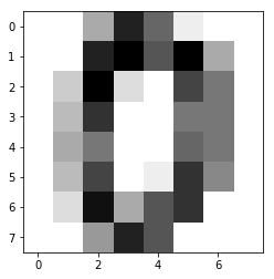
——————————————————–
と、ゼロが表示された。きっと’target’: array([0, 1, 2, …, 8, 9, 8])の始めのゼロがこの画像との組み合わせなんだろう。
——————————————————–
In: digits.target[0]
Out: 0
——————————————————–
と”0”が引き出せた。
要するに、手書き数字データdigitsは、8×8の時に現配列データとして、2^4と4ビットのデータで保管されている。
それとマッチするように、その画像がどの数字なのかという”正解”が、digits.target[]配列に保存されている。
このtarget[]配列に入る要素は、’target_names’: arrayで規定されている([0, 1, 2, 3, 4, 5, 6, 7, 8, 9])であろう。
——————————————————–
いくつの数字と画像が収められているのか?
——————————————————–
In: digits.target.size
Out: 1797
——————————————————–
In: digits.data.size
Out: 115008 (=64 x 1797)
——————————————————–
In: digits.images.size
Out: 115008 (=64 x 1797)
——————————————————–
配列要素の数はlen()関数でチェック
——————————————————–
In: len(digits.data)
Out: 1797
——————————————————–
In: len(digits.images)
Out: 1797
——————————————————–