Bayesian Biostatistics by E Lesaffre & AB Lawson, Chapter 4 学習ノート ???????????????????????
複数のパラメータをベイズ流ではどう扱うのかについての解説である。
たいへんハードな内容で、1日1章とはいかない。完全に理解するのに一ヶ月くらいかかりそう。
この際、慌てずにゆっくり行こう。一通りのプログラムをまずは動かして、何が課題なのかをざくっと理解することととする。
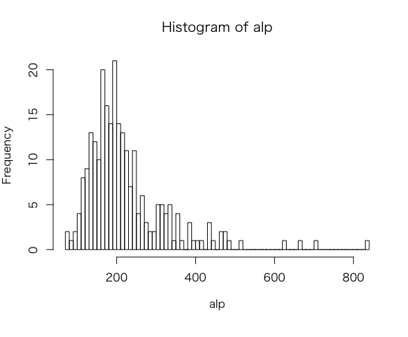
ALP.txtのデータ構造 315個のデータが収納されている。
artikel=0が250個、artikel=1が65個。alkfos[artikel==0]でartikel=0の250件を取り出しているが、残りのartikel=1が何か解らないが、ともかく250件のデータを分析する。
|
1 2 3 4 5 6 7 |
artikel alkfos 0 160 0 263 0 333 0 187 0 220 ..... |
|
1 2 3 4 5 6 7 8 9 10 11 12 13 14 15 16 17 18 |
> attach(ALP) > > alp <- alkfos[artikel==0] > > alp [1] 160 263 333 187 220 200 150 472 166 258 416 203 273 165 144 217 358 190 176 182 [21] 217 114 356 89 203 168 203 265 141 298 139 213 209 327 168 213 145 198 316 267 [41] 228 136 192 835 170 168 159 120 197 395 170 162 249 161 294 362 177 113 139 440 [61] 183 121 308 183 352 167 237 162 390 194 186 143 115 211 708 202 253 196 179 235 [81] 159 135 100 218 211 254 258 178 225 221 182 247 312 117 225 172 109 307 302 106 [101] 308 470 222 200 179 232 244 187 245 134 174 201 203 246 195 187 212 140 185 145 [121] 166 186 249 194 187 467 126 175 144 167 431 130 205 198 138 228 384 169 196 70 [141] 180 147 345 229 245 303 91 200 238 199 194 118 226 174 471 241 332 172 311 137 [161] 316 630 145 101 288 334 243 285 70 229 213 122 279 267 197 404 223 213 209 383 [181] 208 264 144 201 126 212 159 163 322 165 442 324 133 194 234 177 161 279 201 179 [201] 191 270 157 247 124 155 330 206 490 232 131 164 335 435 125 237 360 194 188 144 [221] 128 172 147 225 131 200 108 158 140 113 315 337 178 138 187 157 167 242 153 114 [241] 130 662 194 194 514 175 156 167 213 210 |
|
1 2 3 4 5 6 7 |
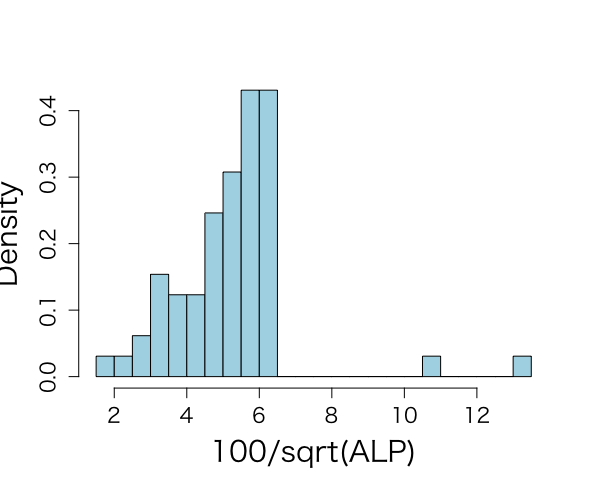
> hist(alp) > mean(alp) [1] 223.852 > var(alp) [1] 11049.13 > sd(alp) [1] 105.1148 |

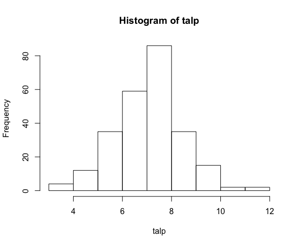
分散の大きさから、明らかに過分散データであるから、以下のように、正規分布に近似される100*√alp と整形している
|
1 2 3 4 5 6 7 8 9 10 11 12 13 14 15 16 17 18 19 20 21 22 23 24 25 26 27 28 29 30 31 32 33 34 |
> talp <- 100*alp^(-1/2) > talp [1] 7.905694 6.166264 5.479966 7.312724 6.741999 7.071068 8.164966 4.602873 [9] 7.761505 6.225728 4.902903 7.018624 6.052275 7.784989 8.333333 6.788442 [17] 5.285164 7.254763 7.537784 7.412493 6.788442 9.365858 5.299989 10.599979 [25] 7.018624 7.715167 7.018624 6.142951 8.421519 5.792844 8.481889 6.851887 [33] 6.917145 5.530013 7.715167 6.851887 8.304548 7.106691 5.625440 6.119901 [41] 6.622662 8.574929 7.216878 3.460643 7.669650 7.715167 7.930516 9.128709 [49] 7.124705 5.031546 7.669650 7.856742 6.337243 7.881104 5.832118 5.255883 [57] 7.516460 9.407209 8.481889 4.767313 7.392213 9.090909 5.698029 7.392213 [65] 5.330018 7.738232 6.495698 7.856742 5.063697 7.179582 7.332356 8.362420 [73] 9.325048 6.884284 3.758230 7.035975 6.286946 7.142857 7.474351 6.523281 [81] 7.930516 8.606630 10.000000 6.772855 6.884284 6.274558 6.225728 7.495317 [89] 6.666667 6.726728 7.412493 6.362848 5.661385 9.245003 6.666667 7.624929 [97] 9.578263 5.707301 5.754353 9.712859 5.698029 4.612656 6.711561 7.071068 [105] 7.474351 6.565322 6.401844 7.312724 6.388766 8.638684 7.580980 7.053456 [113] 7.018624 6.375767 7.161149 7.312724 6.868028 8.451543 7.352146 8.304548 [121] 7.761505 7.332356 6.337243 7.179582 7.312724 4.627448 8.908708 7.559289 [129] 8.333333 7.738232 4.816831 8.770580 6.984303 7.106691 8.512565 6.622662 [137] 5.103104 7.692308 7.142857 11.952286 7.453560 8.247861 5.383819 6.608186 [145] 6.388766 5.744850 10.482848 7.071068 6.482037 7.088812 7.179582 9.205746 [153] 6.651901 7.580980 4.607757 6.441566 5.488213 7.624929 5.670480 8.543577 [161] 5.625440 3.984095 8.304548 9.950372 5.892557 5.471757 6.415003 5.923489 [169] 11.952286 6.608186 6.851887 9.053575 5.986843 6.119901 7.124705 4.975186 [177] 6.696495 6.851887 6.917145 5.109761 6.933752 6.154575 8.333333 7.053456 [185] 8.908708 6.868028 7.930516 7.832604 5.572782 7.784989 4.756515 5.555556 [193] 8.671100 7.179582 6.537205 7.516460 7.881104 5.986843 7.053456 7.474351 [201] 7.235746 6.085806 7.980869 6.362848 8.980265 8.032193 5.504819 6.967330 [209] 4.517540 6.565322 8.737041 7.808688 5.463584 4.794633 8.944272 6.495698 [217] 5.270463 7.179582 7.293250 8.333333 8.838835 7.624929 8.247861 6.666667 [225] 8.737041 7.071068 9.622504 7.955573 8.451543 9.407209 5.634362 5.447347 [233] 7.495317 8.512565 7.312724 7.980869 7.738232 6.428243 8.084521 9.365858 [241] 8.770580 3.886610 7.179582 7.179582 4.410811 7.559289 8.006408 7.738232 [249] 6.851887 6.900656 |
|
1 2 3 4 5 6 7 |
> mean(talp) [1] 7.108724 > sd(talp) [1] 1.365344 > var(talp) [1] 1.864165 > hist(talp) |
頻度論アプローチで、N(μ, σ^2)に関して、観測値yの95%参照区間は、[μ-1.96σ, μ+1.96σ]
y_mean = 7.11で、s = 1.4なので、alpの尺度で95%参照区間は[104.45, 508.95]となるが、
この区間はμを推定するときのばらつきを無視している。yの標本分布を考慮すれば、y-y_mean〜N[0, σ^2(1+1/n)]であり、95%参照区間は[y_mean – 1.96σ√(1+1/n),y_mean + 1.96σ√(1+1/n)]となり、スケール化yは[4.43, 9.79]、もとの値では[104.33, 510.18]となる。
|
1 2 3 4 5 6 7 8 9 10 11 12 13 14 |
> install.packages("lattice") URL 'https://cran.rstudio.com/bin/macosx/el-capitan/contrib/3.4/lattice_0.20-35.tgz' を試しています Content type 'application/x-gzip' length 721744 bytes (704 KB) ================================================== downloaded 704 KB The downloaded binary packages are in /var/folders/0j/j_y5y9pj73g9f1r01zqzycxm0000gp/T//RtmpZgOZcK/downloaded_packages > library(lattice) > attach(ALP) > > objects(2) [1] "alkfos" "artikel" |
y=100/√alpとした同時分布p(μ,σ^2|y)を推測
|
1 2 3 4 5 6 7 8 9 10 11 12 13 14 15 16 17 18 19 20 |
> alp <- alkfos[artikel==0] > talp <- 100*alp^(-1/2) > nalp <- length(alp) > > mtalp <- mean(talp) > vartalp <- var(talp) > sdtalp <- sqrt(var(talp)) > ntalp <- length(talp) > > mtalp;sdtalp [1] 7.108724 [1] 1.365344 > nalp [1] 250 > ntalp [1] 250 > vartalp [1] 1.864165 > hist(alp) > hist(alp, breaks=100) |
|
1 2 3 4 5 6 7 8 |
> par(mfrow=c(1,1)) > par(pty="m") > par(mar=c(5,5,4,2)+0.1) > > # histogram of transformed response, graph is not included in book > > hist(talp,xlab="100/sqrt(ALP)",nclas=30,col="light blue", + cex.lab=1.8,cex.axis=1.3,prob=T,main="") |

|
1 2 3 4 5 6 7 8 9 10 11 12 13 14 15 16 17 18 19 20 21 22 23 24 25 26 27 28 29 30 31 32 33 34 35 36 37 38 39 40 41 42 43 44 45 46 47 48 49 50 51 52 53 54 55 56 57 58 59 60 61 62 63 64 65 66 67 68 69 70 71 72 73 74 75 76 77 78 79 80 81 82 83 84 85 86 87 88 89 90 91 92 93 94 95 96 97 98 99 100 101 102 103 104 105 106 107 108 109 110 111 112 113 114 115 116 117 118 119 120 121 122 123 124 125 126 127 128 129 130 131 132 133 134 135 136 137 138 139 140 141 142 143 144 145 146 147 148 149 150 151 152 153 154 155 156 157 158 159 160 161 162 163 164 165 166 167 168 169 170 171 172 173 174 175 176 177 178 179 180 181 182 183 184 185 186 187 188 189 190 191 192 193 194 195 196 197 198 199 200 201 202 203 204 205 206 |
> # graph of 2-dimensional normal posterior distribution > > unl.mu <- 6.8 > upl.mu <- 7.4 > > unl.sigma2 <- 1.2 > upl.sigma2 <- 2.5 > > # log posterior of mu and sigma2 given y: graph! > > # choice of 200 for calculations, 50 for plotting > > nmu <- 30 > nsigma2 <- 30 > > mugrid <- expand.grid(mu=do.breaks(c(unl.mu,upl.mu),nmu), + sigma2=do.breaks(c(unl.sigma2,upl.sigma2),nsigma2)) > > mugrid$mu [1] 6.80 6.82 6.84 6.86 6.88 6.90 6.92 6.94 6.96 6.98 7.00 7.02 7.04 7.06 7.08 7.10 [17] 7.12 7.14 7.16 7.18 7.20 7.22 7.24 7.26 7.28 7.30 7.32 7.34 7.36 7.38 7.40 6.80 [33] 6.82 6.84 6.86 6.88 6.90 6.92 6.94 6.96 6.98 7.00 7.02 7.04 7.06 7.08 7.10 7.12 [49] 7.14 7.16 7.18 7.20 7.22 7.24 7.26 7.28 7.30 7.32 7.34 7.36 7.38 7.40 6.80 6.82 [65] 6.84 6.86 6.88 6.90 6.92 6.94 6.96 6.98 7.00 7.02 7.04 7.06 7.08 7.10 7.12 7.14 [81] 7.16 7.18 7.20 7.22 7.24 7.26 7.28 7.30 7.32 7.34 7.36 7.38 7.40 6.80 6.82 6.84 [97] 6.86 6.88 6.90 6.92 6.94 6.96 6.98 7.00 7.02 7.04 7.06 7.08 7.10 7.12 7.14 7.16 [113] 7.18 7.20 7.22 7.24 7.26 7.28 7.30 7.32 7.34 7.36 7.38 7.40 6.80 6.82 6.84 6.86 [129] 6.88 6.90 6.92 6.94 6.96 6.98 7.00 7.02 7.04 7.06 7.08 7.10 7.12 7.14 7.16 7.18 [145] 7.20 7.22 7.24 7.26 7.28 7.30 7.32 7.34 7.36 7.38 7.40 6.80 6.82 6.84 6.86 6.88 [161] 6.90 6.92 6.94 6.96 6.98 7.00 7.02 7.04 7.06 7.08 7.10 7.12 7.14 7.16 7.18 7.20 [177] 7.22 7.24 7.26 7.28 7.30 7.32 7.34 7.36 7.38 7.40 6.80 6.82 6.84 6.86 6.88 6.90 [193] 6.92 6.94 6.96 6.98 7.00 7.02 7.04 7.06 7.08 7.10 7.12 7.14 7.16 7.18 7.20 7.22 [209] 7.24 7.26 7.28 7.30 7.32 7.34 7.36 7.38 7.40 6.80 6.82 6.84 6.86 6.88 6.90 6.92 [225] 6.94 6.96 6.98 7.00 7.02 7.04 7.06 7.08 7.10 7.12 7.14 7.16 7.18 7.20 7.22 7.24 [241] 7.26 7.28 7.30 7.32 7.34 7.36 7.38 7.40 6.80 6.82 6.84 6.86 6.88 6.90 6.92 6.94 [257] 6.96 6.98 7.00 7.02 7.04 7.06 7.08 7.10 7.12 7.14 7.16 7.18 7.20 7.22 7.24 7.26 [273] 7.28 7.30 7.32 7.34 7.36 7.38 7.40 6.80 6.82 6.84 6.86 6.88 6.90 6.92 6.94 6.96 [289] 6.98 7.00 7.02 7.04 7.06 7.08 7.10 7.12 7.14 7.16 7.18 7.20 7.22 7.24 7.26 7.28 [305] 7.30 7.32 7.34 7.36 7.38 7.40 6.80 6.82 6.84 6.86 6.88 6.90 6.92 6.94 6.96 6.98 [321] 7.00 7.02 7.04 7.06 7.08 7.10 7.12 7.14 7.16 7.18 7.20 7.22 7.24 7.26 7.28 7.30 [337] 7.32 7.34 7.36 7.38 7.40 6.80 6.82 6.84 6.86 6.88 6.90 6.92 6.94 6.96 6.98 7.00 [353] 7.02 7.04 7.06 7.08 7.10 7.12 7.14 7.16 7.18 7.20 7.22 7.24 7.26 7.28 7.30 7.32 [369] 7.34 7.36 7.38 7.40 6.80 6.82 6.84 6.86 6.88 6.90 6.92 6.94 6.96 6.98 7.00 7.02 [385] 7.04 7.06 7.08 7.10 7.12 7.14 7.16 7.18 7.20 7.22 7.24 7.26 7.28 7.30 7.32 7.34 [401] 7.36 7.38 7.40 6.80 6.82 6.84 6.86 6.88 6.90 6.92 6.94 6.96 6.98 7.00 7.02 7.04 [417] 7.06 7.08 7.10 7.12 7.14 7.16 7.18 7.20 7.22 7.24 7.26 7.28 7.30 7.32 7.34 7.36 [433] 7.38 7.40 6.80 6.82 6.84 6.86 6.88 6.90 6.92 6.94 6.96 6.98 7.00 7.02 7.04 7.06 [449] 7.08 7.10 7.12 7.14 7.16 7.18 7.20 7.22 7.24 7.26 7.28 7.30 7.32 7.34 7.36 7.38 [465] 7.40 6.80 6.82 6.84 6.86 6.88 6.90 6.92 6.94 6.96 6.98 7.00 7.02 7.04 7.06 7.08 [481] 7.10 7.12 7.14 7.16 7.18 7.20 7.22 7.24 7.26 7.28 7.30 7.32 7.34 7.36 7.38 7.40 [497] 6.80 6.82 6.84 6.86 6.88 6.90 6.92 6.94 6.96 6.98 7.00 7.02 7.04 7.06 7.08 7.10 [513] 7.12 7.14 7.16 7.18 7.20 7.22 7.24 7.26 7.28 7.30 7.32 7.34 7.36 7.38 7.40 6.80 [529] 6.82 6.84 6.86 6.88 6.90 6.92 6.94 6.96 6.98 7.00 7.02 7.04 7.06 7.08 7.10 7.12 [545] 7.14 7.16 7.18 7.20 7.22 7.24 7.26 7.28 7.30 7.32 7.34 7.36 7.38 7.40 6.80 6.82 [561] 6.84 6.86 6.88 6.90 6.92 6.94 6.96 6.98 7.00 7.02 7.04 7.06 7.08 7.10 7.12 7.14 [577] 7.16 7.18 7.20 7.22 7.24 7.26 7.28 7.30 7.32 7.34 7.36 7.38 7.40 6.80 6.82 6.84 [593] 6.86 6.88 6.90 6.92 6.94 6.96 6.98 7.00 7.02 7.04 7.06 7.08 7.10 7.12 7.14 7.16 [609] 7.18 7.20 7.22 7.24 7.26 7.28 7.30 7.32 7.34 7.36 7.38 7.40 6.80 6.82 6.84 6.86 [625] 6.88 6.90 6.92 6.94 6.96 6.98 7.00 7.02 7.04 7.06 7.08 7.10 7.12 7.14 7.16 7.18 [641] 7.20 7.22 7.24 7.26 7.28 7.30 7.32 7.34 7.36 7.38 7.40 6.80 6.82 6.84 6.86 6.88 [657] 6.90 6.92 6.94 6.96 6.98 7.00 7.02 7.04 7.06 7.08 7.10 7.12 7.14 7.16 7.18 7.20 [673] 7.22 7.24 7.26 7.28 7.30 7.32 7.34 7.36 7.38 7.40 6.80 6.82 6.84 6.86 6.88 6.90 [689] 6.92 6.94 6.96 6.98 7.00 7.02 7.04 7.06 7.08 7.10 7.12 7.14 7.16 7.18 7.20 7.22 [705] 7.24 7.26 7.28 7.30 7.32 7.34 7.36 7.38 7.40 6.80 6.82 6.84 6.86 6.88 6.90 6.92 [721] 6.94 6.96 6.98 7.00 7.02 7.04 7.06 7.08 7.10 7.12 7.14 7.16 7.18 7.20 7.22 7.24 [737] 7.26 7.28 7.30 7.32 7.34 7.36 7.38 7.40 6.80 6.82 6.84 6.86 6.88 6.90 6.92 6.94 [753] 6.96 6.98 7.00 7.02 7.04 7.06 7.08 7.10 7.12 7.14 7.16 7.18 7.20 7.22 7.24 7.26 [769] 7.28 7.30 7.32 7.34 7.36 7.38 7.40 6.80 6.82 6.84 6.86 6.88 6.90 6.92 6.94 6.96 [785] 6.98 7.00 7.02 7.04 7.06 7.08 7.10 7.12 7.14 7.16 7.18 7.20 7.22 7.24 7.26 7.28 [801] 7.30 7.32 7.34 7.36 7.38 7.40 6.80 6.82 6.84 6.86 6.88 6.90 6.92 6.94 6.96 6.98 [817] 7.00 7.02 7.04 7.06 7.08 7.10 7.12 7.14 7.16 7.18 7.20 7.22 7.24 7.26 7.28 7.30 [833] 7.32 7.34 7.36 7.38 7.40 6.80 6.82 6.84 6.86 6.88 6.90 6.92 6.94 6.96 6.98 7.00 [849] 7.02 7.04 7.06 7.08 7.10 7.12 7.14 7.16 7.18 7.20 7.22 7.24 7.26 7.28 7.30 7.32 [865] 7.34 7.36 7.38 7.40 6.80 6.82 6.84 6.86 6.88 6.90 6.92 6.94 6.96 6.98 7.00 7.02 [881] 7.04 7.06 7.08 7.10 7.12 7.14 7.16 7.18 7.20 7.22 7.24 7.26 7.28 7.30 7.32 7.34 [897] 7.36 7.38 7.40 6.80 6.82 6.84 6.86 6.88 6.90 6.92 6.94 6.96 6.98 7.00 7.02 7.04 [913] 7.06 7.08 7.10 7.12 7.14 7.16 7.18 7.20 7.22 7.24 7.26 7.28 7.30 7.32 7.34 7.36 [929] 7.38 7.40 6.80 6.82 6.84 6.86 6.88 6.90 6.92 6.94 6.96 6.98 7.00 7.02 7.04 7.06 [945] 7.08 7.10 7.12 7.14 7.16 7.18 7.20 7.22 7.24 7.26 7.28 7.30 7.32 7.34 7.36 7.38 [961] 7.40 > mugrid$sigma2 [1] 1.200000 1.200000 1.200000 1.200000 1.200000 1.200000 1.200000 1.200000 1.200000 [10] 1.200000 1.200000 1.200000 1.200000 1.200000 1.200000 1.200000 1.200000 1.200000 [19] 1.200000 1.200000 1.200000 1.200000 1.200000 1.200000 1.200000 1.200000 1.200000 [28] 1.200000 1.200000 1.200000 1.200000 1.243333 1.243333 1.243333 1.243333 1.243333 [37] 1.243333 1.243333 1.243333 1.243333 1.243333 1.243333 1.243333 1.243333 1.243333 [46] 1.243333 1.243333 1.243333 1.243333 1.243333 1.243333 1.243333 1.243333 1.243333 [55] 1.243333 1.243333 1.243333 1.243333 1.243333 1.243333 1.243333 1.243333 1.286667 [64] 1.286667 1.286667 1.286667 1.286667 1.286667 1.286667 1.286667 1.286667 1.286667 [73] 1.286667 1.286667 1.286667 1.286667 1.286667 1.286667 1.286667 1.286667 1.286667 [82] 1.286667 1.286667 1.286667 1.286667 1.286667 1.286667 1.286667 1.286667 1.286667 [91] 1.286667 1.286667 1.286667 1.330000 1.330000 1.330000 1.330000 1.330000 1.330000 [100] 1.330000 1.330000 1.330000 1.330000 1.330000 1.330000 1.330000 1.330000 1.330000 [109] 1.330000 1.330000 1.330000 1.330000 1.330000 1.330000 1.330000 1.330000 1.330000 [118] 1.330000 1.330000 1.330000 1.330000 1.330000 1.330000 1.330000 1.373333 1.373333 [127] 1.373333 1.373333 1.373333 1.373333 1.373333 1.373333 1.373333 1.373333 1.373333 [136] 1.373333 1.373333 1.373333 1.373333 1.373333 1.373333 1.373333 1.373333 1.373333 [145] 1.373333 1.373333 1.373333 1.373333 1.373333 1.373333 1.373333 1.373333 1.373333 [154] 1.373333 1.373333 1.416667 1.416667 1.416667 1.416667 1.416667 1.416667 1.416667 [163] 1.416667 1.416667 1.416667 1.416667 1.416667 1.416667 1.416667 1.416667 1.416667 [172] 1.416667 1.416667 1.416667 1.416667 1.416667 1.416667 1.416667 1.416667 1.416667 [181] 1.416667 1.416667 1.416667 1.416667 1.416667 1.416667 1.460000 1.460000 1.460000 [190] 1.460000 1.460000 1.460000 1.460000 1.460000 1.460000 1.460000 1.460000 1.460000 [199] 1.460000 1.460000 1.460000 1.460000 1.460000 1.460000 1.460000 1.460000 1.460000 [208] 1.460000 1.460000 1.460000 1.460000 1.460000 1.460000 1.460000 1.460000 1.460000 [217] 1.460000 1.503333 1.503333 1.503333 1.503333 1.503333 1.503333 1.503333 1.503333 [226] 1.503333 1.503333 1.503333 1.503333 1.503333 1.503333 1.503333 1.503333 1.503333 [235] 1.503333 1.503333 1.503333 1.503333 1.503333 1.503333 1.503333 1.503333 1.503333 [244] 1.503333 1.503333 1.503333 1.503333 1.503333 1.546667 1.546667 1.546667 1.546667 [253] 1.546667 1.546667 1.546667 1.546667 1.546667 1.546667 1.546667 1.546667 1.546667 [262] 1.546667 1.546667 1.546667 1.546667 1.546667 1.546667 1.546667 1.546667 1.546667 [271] 1.546667 1.546667 1.546667 1.546667 1.546667 1.546667 1.546667 1.546667 1.546667 [280] 1.590000 1.590000 1.590000 1.590000 1.590000 1.590000 1.590000 1.590000 1.590000 [289] 1.590000 1.590000 1.590000 1.590000 1.590000 1.590000 1.590000 1.590000 1.590000 [298] 1.590000 1.590000 1.590000 1.590000 1.590000 1.590000 1.590000 1.590000 1.590000 [307] 1.590000 1.590000 1.590000 1.590000 1.633333 1.633333 1.633333 1.633333 1.633333 [316] 1.633333 1.633333 1.633333 1.633333 1.633333 1.633333 1.633333 1.633333 1.633333 [325] 1.633333 1.633333 1.633333 1.633333 1.633333 1.633333 1.633333 1.633333 1.633333 [334] 1.633333 1.633333 1.633333 1.633333 1.633333 1.633333 1.633333 1.633333 1.676667 [343] 1.676667 1.676667 1.676667 1.676667 1.676667 1.676667 1.676667 1.676667 1.676667 [352] 1.676667 1.676667 1.676667 1.676667 1.676667 1.676667 1.676667 1.676667 1.676667 [361] 1.676667 1.676667 1.676667 1.676667 1.676667 1.676667 1.676667 1.676667 1.676667 [370] 1.676667 1.676667 1.676667 1.720000 1.720000 1.720000 1.720000 1.720000 1.720000 [379] 1.720000 1.720000 1.720000 1.720000 1.720000 1.720000 1.720000 1.720000 1.720000 [388] 1.720000 1.720000 1.720000 1.720000 1.720000 1.720000 1.720000 1.720000 1.720000 [397] 1.720000 1.720000 1.720000 1.720000 1.720000 1.720000 1.720000 1.763333 1.763333 [406] 1.763333 1.763333 1.763333 1.763333 1.763333 1.763333 1.763333 1.763333 1.763333 [415] 1.763333 1.763333 1.763333 1.763333 1.763333 1.763333 1.763333 1.763333 1.763333 [424] 1.763333 1.763333 1.763333 1.763333 1.763333 1.763333 1.763333 1.763333 1.763333 [433] 1.763333 1.763333 1.806667 1.806667 1.806667 1.806667 1.806667 1.806667 1.806667 [442] 1.806667 1.806667 1.806667 1.806667 1.806667 1.806667 1.806667 1.806667 1.806667 [451] 1.806667 1.806667 1.806667 1.806667 1.806667 1.806667 1.806667 1.806667 1.806667 [460] 1.806667 1.806667 1.806667 1.806667 1.806667 1.806667 1.850000 1.850000 1.850000 [469] 1.850000 1.850000 1.850000 1.850000 1.850000 1.850000 1.850000 1.850000 1.850000 [478] 1.850000 1.850000 1.850000 1.850000 1.850000 1.850000 1.850000 1.850000 1.850000 [487] 1.850000 1.850000 1.850000 1.850000 1.850000 1.850000 1.850000 1.850000 1.850000 [496] 1.850000 1.893333 1.893333 1.893333 1.893333 1.893333 1.893333 1.893333 1.893333 [505] 1.893333 1.893333 1.893333 1.893333 1.893333 1.893333 1.893333 1.893333 1.893333 [514] 1.893333 1.893333 1.893333 1.893333 1.893333 1.893333 1.893333 1.893333 1.893333 [523] 1.893333 1.893333 1.893333 1.893333 1.893333 1.936667 1.936667 1.936667 1.936667 [532] 1.936667 1.936667 1.936667 1.936667 1.936667 1.936667 1.936667 1.936667 1.936667 [541] 1.936667 1.936667 1.936667 1.936667 1.936667 1.936667 1.936667 1.936667 1.936667 [550] 1.936667 1.936667 1.936667 1.936667 1.936667 1.936667 1.936667 1.936667 1.936667 [559] 1.980000 1.980000 1.980000 1.980000 1.980000 1.980000 1.980000 1.980000 1.980000 [568] 1.980000 1.980000 1.980000 1.980000 1.980000 1.980000 1.980000 1.980000 1.980000 [577] 1.980000 1.980000 1.980000 1.980000 1.980000 1.980000 1.980000 1.980000 1.980000 [586] 1.980000 1.980000 1.980000 1.980000 2.023333 2.023333 2.023333 2.023333 2.023333 [595] 2.023333 2.023333 2.023333 2.023333 2.023333 2.023333 2.023333 2.023333 2.023333 [604] 2.023333 2.023333 2.023333 2.023333 2.023333 2.023333 2.023333 2.023333 2.023333 [613] 2.023333 2.023333 2.023333 2.023333 2.023333 2.023333 2.023333 2.023333 2.066667 [622] 2.066667 2.066667 2.066667 2.066667 2.066667 2.066667 2.066667 2.066667 2.066667 [631] 2.066667 2.066667 2.066667 2.066667 2.066667 2.066667 2.066667 2.066667 2.066667 [640] 2.066667 2.066667 2.066667 2.066667 2.066667 2.066667 2.066667 2.066667 2.066667 [649] 2.066667 2.066667 2.066667 2.110000 2.110000 2.110000 2.110000 2.110000 2.110000 [658] 2.110000 2.110000 2.110000 2.110000 2.110000 2.110000 2.110000 2.110000 2.110000 [667] 2.110000 2.110000 2.110000 2.110000 2.110000 2.110000 2.110000 2.110000 2.110000 [676] 2.110000 2.110000 2.110000 2.110000 2.110000 2.110000 2.110000 2.153333 2.153333 [685] 2.153333 2.153333 2.153333 2.153333 2.153333 2.153333 2.153333 2.153333 2.153333 [694] 2.153333 2.153333 2.153333 2.153333 2.153333 2.153333 2.153333 2.153333 2.153333 [703] 2.153333 2.153333 2.153333 2.153333 2.153333 2.153333 2.153333 2.153333 2.153333 [712] 2.153333 2.153333 2.196667 2.196667 2.196667 2.196667 2.196667 2.196667 2.196667 [721] 2.196667 2.196667 2.196667 2.196667 2.196667 2.196667 2.196667 2.196667 2.196667 [730] 2.196667 2.196667 2.196667 2.196667 2.196667 2.196667 2.196667 2.196667 2.196667 [739] 2.196667 2.196667 2.196667 2.196667 2.196667 2.196667 2.240000 2.240000 2.240000 [748] 2.240000 2.240000 2.240000 2.240000 2.240000 2.240000 2.240000 2.240000 2.240000 [757] 2.240000 2.240000 2.240000 2.240000 2.240000 2.240000 2.240000 2.240000 2.240000 [766] 2.240000 2.240000 2.240000 2.240000 2.240000 2.240000 2.240000 2.240000 2.240000 [775] 2.240000 2.283333 2.283333 2.283333 2.283333 2.283333 2.283333 2.283333 2.283333 [784] 2.283333 2.283333 2.283333 2.283333 2.283333 2.283333 2.283333 2.283333 2.283333 [793] 2.283333 2.283333 2.283333 2.283333 2.283333 2.283333 2.283333 2.283333 2.283333 [802] 2.283333 2.283333 2.283333 2.283333 2.283333 2.326667 2.326667 2.326667 2.326667 [811] 2.326667 2.326667 2.326667 2.326667 2.326667 2.326667 2.326667 2.326667 2.326667 [820] 2.326667 2.326667 2.326667 2.326667 2.326667 2.326667 2.326667 2.326667 2.326667 [829] 2.326667 2.326667 2.326667 2.326667 2.326667 2.326667 2.326667 2.326667 2.326667 [838] 2.370000 2.370000 2.370000 2.370000 2.370000 2.370000 2.370000 2.370000 2.370000 [847] 2.370000 2.370000 2.370000 2.370000 2.370000 2.370000 2.370000 2.370000 2.370000 [856] 2.370000 2.370000 2.370000 2.370000 2.370000 2.370000 2.370000 2.370000 2.370000 [865] 2.370000 2.370000 2.370000 2.370000 2.413333 2.413333 2.413333 2.413333 2.413333 [874] 2.413333 2.413333 2.413333 2.413333 2.413333 2.413333 2.413333 2.413333 2.413333 [883] 2.413333 2.413333 2.413333 2.413333 2.413333 2.413333 2.413333 2.413333 2.413333 [892] 2.413333 2.413333 2.413333 2.413333 2.413333 2.413333 2.413333 2.413333 2.456667 [901] 2.456667 2.456667 2.456667 2.456667 2.456667 2.456667 2.456667 2.456667 2.456667 [910] 2.456667 2.456667 2.456667 2.456667 2.456667 2.456667 2.456667 2.456667 2.456667 [919] 2.456667 2.456667 2.456667 2.456667 2.456667 2.456667 2.456667 2.456667 2.456667 [928] 2.456667 2.456667 2.456667 2.500000 2.500000 2.500000 2.500000 2.500000 2.500000 [937] 2.500000 2.500000 2.500000 2.500000 2.500000 2.500000 2.500000 2.500000 2.500000 [946] 2.500000 2.500000 2.500000 2.500000 2.500000 2.500000 2.500000 2.500000 2.500000 [955] 2.500000 2.500000 2.500000 2.500000 2.500000 2.500000 2.500000 > > logpropposter <- -(ntalp+2)*log(mugrid$sigma2)/2 > logpropposter <- logpropposter -0.5*mugrid$sigma2^(-1)*((ntalp-1)*vartalp+ntalp*(mtalp-mugrid$mu)^2) > propposter <- exp(logpropposter-max(logpropposter)) > > par(mfrow=c(1,1)) > par(pty="m") > par(mar=c(6,4,4,2)) > trellis.par.set("axis.line",list(col="transparent")) > wireframe(propposter ~ mugrid$mu*mugrid$sigma2,outer=TRUE, + shade=TRUE,bty="l",zlab="", + xlab=list(label=expression(paste(mu)),font=1,cex=1.8), + ylab=list(label=expression(paste(sigma^{2})),font=1,cex=1.8), + scales = list(arrows=FALSE, cex= 1.2, col = "black",font = 3, + z = list(draw = FALSE)), + par.box = list(col=NA), + shade.colors = function(irr, ref, height, w = 1) + grey(w * irr + (1 - w) * (1 - (1 - ref)^0.4)),zoom=1) |
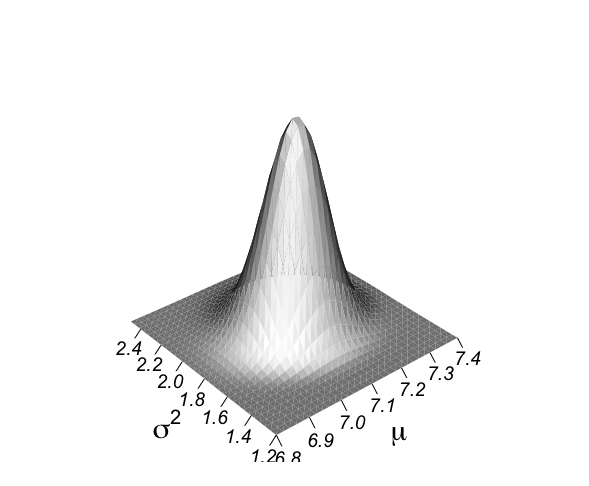
と、美しい三次元立体図が描けた。
mugrid$muとmugrid$sigma2が、xy座標のパラメータで、z座標がヒストグラム頻度であろう。
mugridを排出するexpand.grid()関数とは何か?
|
1 |
> ?expand.grid() |
expand.grid {base} R Documentation
Create a Data Frame from All Combinations of Factor Variables
Description
Create a data frame from all combinations of the supplied vectors or factors. See the description of the return value for precise details of the way this is done.
Usage
expand.grid(…, KEEP.OUT.ATTRS = TRUE, stringsAsFactors = TRUE)
Arguments
…
vectors, factors or a list containing these.
KEEP.OUT.ATTRS
a logical indicating the “out.attrs” attribute (see below) should be computed and returned.
stringsAsFactors
logical specifying if character vectors are converted to factors.
Value
A data frame containing one row for each combination of the supplied factors. The first factors vary fastest. The columns are labelled by the factors if these are supplied as named arguments or named components of a list. The row names are ‘automatic’.
Attribute “out.attrs” is a list which gives the dimension and dimnames for use by predict methods.
Note
Conversion to a factor is done with levels in the order they occur in the character vectors (and not alphabetically, as is most common when converting to factors).
References
Chambers, J. M. and Hastie, T. J. (1992) Statistical Models in S. Wadsworth & Brooks/Cole.
See Also
combn (package utils) for the generation of all combinations of n elements, taken m at a time.
Examples
require(utils)
expand.grid(height = seq(60, 80, 5), weight = seq(100, 300, 50),
sex = c(“Male”,”Female”))
x <- seq(0, 10, length.out = 100)
y <- seq(-1, 1, length.out = 20)
d1 <- expand.grid(x = x, y = y)
d2 <- expand.grid(x = x, y = y, KEEP.OUT.ATTRS = FALSE)
object.size(d1) - object.size(d2)
##-> 5992 or 8832 (on 32- / 64-bit platform)
ーーーーーーーーーーーーーーーーーーーーーー
|
1 2 |
> mugrid <- expand.grid(mu=do.breaks(c(unl.mu,upl.mu),nmu), + sigma2=do.breaks(c(unl.sigma2,upl.sigma2),nsigma2)) |
は何をしているのか?
サンプルデータの作成:関数 expand.grid()
関数 expand.grid(引数1=ベクトル1,引数2=ベクトル2,・・・) を用いることで,引数に指定した因子全ての組み合わせから成るデータフレームを作ることができる.
expand.grid関数を使って、引数のベクトルの全組み合わせを作ることができます。例えば、こんな風に作れます。
Rコンソール
> expand.grid(1:2,1:3)
Var1 Var2
1 1 1
2 2 1
3 1 2
4 2 2
5 1 3
6 2 3
|
1 2 3 4 5 6 |
> mugrid mu sigma2 1 6.80 1.200000 2 6.82 1.200000 3 6.84 1.200000 4 6.86 1.200000 |
expand.grid()の中身を見てみる。
mu=do.breaks(c(unl.mu,upl.mu),nmu),
sigma2=do.breaks(c(unl.sigma2,upl.sigma2),nsigma2)
|
1 2 3 4 5 6 7 8 9 10 11 12 |
> unl.mu <- 6.8 > upl.mu <- 7.4 > > unl.sigma2 <- 1.2 > upl.sigma2 <- 2.5 > > # log posterior of mu and sigma2 given y: graph! > > # choice of 200 for calculations, 50 for plotting > > nmu <- 30 > nsigma2 <- 30 |
平均が7.1なので、7.1 ± 0.3をunl.mu, up1.muとしているようだ。
分散は1.86、標準偏差は分散のルートで1.36。
unl.sigma2 <- 1.2, upl.sigma2 <- 2.5がどこから来たのかわからない。
|
1 2 3 4 5 6 7 8 9 10 11 12 13 |
mu=do.breaks(c(6.8,7.4),30), sigma2=do.breaks(c(1.2,2.5),30) > mu=do.breaks(c(6.8,7.4),30) > mu [1] 6.80 6.82 6.84 6.86 6.88 6.90 6.92 6.94 6.96 6.98 7.00 7.02 7.04 7.06 7.08 7.10 [17] 7.12 7.14 7.16 7.18 7.20 7.22 7.24 7.26 7.28 7.30 7.32 7.34 7.36 7.38 7.40 > sigma2=do.breaks(c(1.2,2.5),30) > sigma2 [1] 1.200000 1.243333 1.286667 1.330000 1.373333 1.416667 1.460000 1.503333 1.546667 [10] 1.590000 1.633333 1.676667 1.720000 1.763333 1.806667 1.850000 1.893333 1.936667 [19] 1.980000 2.023333 2.066667 2.110000 2.153333 2.196667 2.240000 2.283333 2.326667 [28] 2.370000 2.413333 2.456667 2.500000 |
次のパッケージでは、
|
1 2 3 4 5 6 7 8 9 10 11 12 13 14 15 16 17 18 19 20 21 22 23 24 25 26 27 28 29 30 31 32 33 34 35 36 37 38 39 40 41 42 43 44 45 |
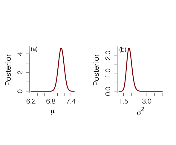
> library(lattice) > attach(ALP) > > objects(2) [1] "alkfos" "artikel" > > alp <- alkfos[artikel==0] > talp <- 100*alp^(-1/2) > nalp <- length(alp) > > mtalp <- mean(talp) > vartalp <- var(talp) > sdtalp <- sqrt(var(talp)) > ntalp <- length(talp) > > mtalp;sdtalp [1] 7.108724 [1] 1.365344 > > par(mfrow=c(1,1)) > par(pty="m") > par(mar=c(5,5,4,2)+0.1) > > > # marginal posterior distribution of MEAN & SIGMAイ > # Figure 4.2 but only part of ninf prior > > > unl.mu <- 6.2 > upl.mu <- 7.5 > > unl.sigma2 <- 1.2 > upl.sigma2 <- 4 > > nmu <- 100 > nsigma2 <- 100 > > # values using ni prior > > mu <- seq(unl.mu,upl.mu,length=nmu) > mus <- (mu-mtalp)/(sdtalp/sqrt(ntalp)) > pmu <- dt(mus,ntalp-1)*sqrt(ntalp)/sdtalp > sigma2 <- seq(unl.sigma2,upl.sigma2,length=nsigma2) > sigma2s <- (ntalp-1)*vartalp/sigma2 > psigma2 <- dchisq(sigma2s,ntalp-1)*(ntalp-1)*vartalp/(sigma2^2) |
mu <- seq(6.2,7.5,length=100) mus <- (mu-7.1)/(σ/sqrt(n)) pmu <- dt(mus,n-1)*sqrt(n)/σ sigma2 <- seq(1.2,4,length=100) sigma2s <- (n-1)*var/σ2 psigma2 <- dchisq(sigma2s,n-1)*(n-1)*var/(σ2^2)
|
1 2 3 4 5 6 7 8 9 10 11 12 13 14 15 16 17 18 19 20 21 22 23 24 25 26 27 28 29 30 31 32 33 34 35 36 37 38 39 40 41 42 43 44 45 46 47 48 49 50 51 52 53 54 55 56 57 58 59 60 61 62 63 64 65 66 67 68 69 70 71 72 73 74 75 76 77 78 79 80 81 82 83 84 85 86 87 88 89 90 91 92 93 94 95 96 97 98 99 100 101 102 103 104 105 106 107 |
> mu [1] 6.200000 6.213131 6.226263 6.239394 6.252525 6.265657 6.278788 6.291919 6.305051 [10] 6.318182 6.331313 6.344444 6.357576 6.370707 6.383838 6.396970 6.410101 6.423232 [19] 6.436364 6.449495 6.462626 6.475758 6.488889 6.502020 6.515152 6.528283 6.541414 [28] 6.554545 6.567677 6.580808 6.593939 6.607071 6.620202 6.633333 6.646465 6.659596 [37] 6.672727 6.685859 6.698990 6.712121 6.725253 6.738384 6.751515 6.764646 6.777778 [46] 6.790909 6.804040 6.817172 6.830303 6.843434 6.856566 6.869697 6.882828 6.895960 [55] 6.909091 6.922222 6.935354 6.948485 6.961616 6.974747 6.987879 7.001010 7.014141 [64] 7.027273 7.040404 7.053535 7.066667 7.079798 7.092929 7.106061 7.119192 7.132323 [73] 7.145455 7.158586 7.171717 7.184848 7.197980 7.211111 7.224242 7.237374 7.250505 [82] 7.263636 7.276768 7.289899 7.303030 7.316162 7.329293 7.342424 7.355556 7.368687 [91] 7.381818 7.394949 7.408081 7.421212 7.434343 7.447475 7.460606 7.473737 7.486869 [100] 7.500000 > mus [1] -10.52348902 -10.37142165 -10.21935428 -10.06728691 -9.91521953 -9.76315216 [7] -9.61108479 -9.45901742 -9.30695005 -9.15488268 -9.00281531 -8.85074794 [13] -8.69868057 -8.54661319 -8.39454582 -8.24247845 -8.09041108 -7.93834371 [19] -7.78627634 -7.63420897 -7.48214160 -7.33007422 -7.17800685 -7.02593948 [25] -6.87387211 -6.72180474 -6.56973737 -6.41767000 -6.26560263 -6.11353526 [31] -5.96146788 -5.80940051 -5.65733314 -5.50526577 -5.35319840 -5.20113103 [37] -5.04906366 -4.89699629 -4.74492891 -4.59286154 -4.44079417 -4.28872680 [43] -4.13665943 -3.98459206 -3.83252469 -3.68045732 -3.52838994 -3.37632257 [49] -3.22425520 -3.07218783 -2.92012046 -2.76805309 -2.61598572 -2.46391835 [55] -2.31185098 -2.15978360 -2.00771623 -1.85564886 -1.70358149 -1.55151412 [61] -1.39944675 -1.24737938 -1.09531201 -0.94324463 -0.79117726 -0.63910989 [67] -0.48704252 -0.33497515 -0.18290778 -0.03084041 0.12122696 0.27329433 [73] 0.42536171 0.57742908 0.72949645 0.88156382 1.03363119 1.18569856 [79] 1.33776593 1.48983330 1.64190068 1.79396805 1.94603542 2.09810279 [85] 2.25017016 2.40223753 2.55430490 2.70637227 2.85843964 3.01050702 [91] 3.16257439 3.31464176 3.46670913 3.61877650 3.77084387 3.92291124 [97] 4.07497861 4.22704599 4.37911336 4.53118073 > pmu [1] 4.897251e-20 1.484466e-19 4.470900e-19 1.337562e-18 3.973860e-18 1.172127e-17 [7] 3.431484e-17 9.968154e-17 2.872442e-16 8.208584e-16 2.325631e-15 6.530436e-15 [13] 1.816956e-14 5.007467e-14 1.366570e-13 3.691934e-13 9.870749e-13 2.610874e-12 [19] 6.830069e-12 1.766570e-11 4.516120e-11 1.140748e-10 2.846194e-10 7.012121e-10 [25] 1.705312e-09 4.092481e-09 9.688500e-09 2.261892e-08 5.205846e-08 1.180791e-07 [31] 2.638616e-07 5.807107e-07 1.258298e-06 2.683539e-06 5.631111e-06 1.162263e-05 [37] 2.358861e-05 4.706009e-05 9.226176e-05 1.776959e-04 3.361163e-04 6.242090e-04 [43] 1.137818e-03 2.035141e-03 3.570870e-03 6.144590e-03 1.036659e-02 1.714316e-02 [49] 2.778103e-02 4.410653e-02 6.858867e-02 1.044476e-01 1.557209e-01 2.272518e-01 [55] 3.245588e-01 4.535481e-01 6.200404e-01 8.291072e-01 1.084245e+00 1.386460e+00 [61] 1.733373e+00 2.118503e+00 2.530873e+00 2.955109e+00 3.372108e+00 3.760299e+00 [67] 4.097416e+00 4.362584e+00 4.538460e+00 4.613118e+00 4.581398e+00 4.445499e+00 [73] 4.214727e+00 3.904430e+00 3.534300e+00 3.126303e+00 2.702525e+00 2.283257e+00 [79] 1.885498e+00 1.522052e+00 1.201202e+00 9.269183e-01 6.994662e-01 5.162475e-01 [85] 3.727226e-01 2.632847e-01 1.819942e-01 1.231306e-01 8.155287e-02 5.288963e-02 [91] 3.359359e-02 2.090247e-02 1.274377e-02 7.614927e-03 4.460788e-03 2.562417e-03 [97] 1.443768e-03 7.981314e-04 4.330155e-04 2.306266e-04 > sigma2 [1] 1.200000 1.228283 1.256566 1.284848 1.313131 1.341414 1.369697 1.397980 1.426263 [10] 1.454545 1.482828 1.511111 1.539394 1.567677 1.595960 1.624242 1.652525 1.680808 [19] 1.709091 1.737374 1.765657 1.793939 1.822222 1.850505 1.878788 1.907071 1.935354 [28] 1.963636 1.991919 2.020202 2.048485 2.076768 2.105051 2.133333 2.161616 2.189899 [37] 2.218182 2.246465 2.274747 2.303030 2.331313 2.359596 2.387879 2.416162 2.444444 [46] 2.472727 2.501010 2.529293 2.557576 2.585859 2.614141 2.642424 2.670707 2.698990 [55] 2.727273 2.755556 2.783838 2.812121 2.840404 2.868687 2.896970 2.925253 2.953535 [64] 2.981818 3.010101 3.038384 3.066667 3.094949 3.123232 3.151515 3.179798 3.208081 [73] 3.236364 3.264646 3.292929 3.321212 3.349495 3.377778 3.406061 3.434343 3.462626 [82] 3.490909 3.519192 3.547475 3.575758 3.604040 3.632323 3.660606 3.688889 3.717172 [91] 3.745455 3.773737 3.802020 3.830303 3.858586 3.886869 3.915152 3.943434 3.971717 [100] 4.000000 > sigma2s [1] 386.8141 377.9072 369.4013 361.2698 353.4886 346.0355 338.8903 332.0341 325.4499 [10] 319.1217 313.0349 307.1759 301.5323 296.0923 290.8451 285.7806 280.8895 276.1630 [19] 271.5929 267.1716 262.8920 258.7473 254.7313 250.8380 247.0619 243.3979 239.8409 [28] 236.3864 233.0300 229.7676 226.5953 223.5093 220.5063 217.5830 214.7361 211.9627 [37] 209.2601 206.6255 204.0565 201.5505 199.1054 196.7188 194.3888 192.1134 189.8906 [46] 187.7186 185.5958 183.5204 181.4910 179.5059 177.5638 175.6633 173.8030 171.9817 [55] 170.1982 168.4513 166.7399 165.0629 163.4193 161.8082 160.2285 158.6793 157.1598 [64] 155.6691 154.2064 152.7710 151.3621 149.9789 148.6207 147.2869 145.9769 144.6899 [73] 143.4255 142.1829 140.9617 139.7613 138.5812 137.4208 136.2797 135.1574 134.0534 [82] 132.9674 131.8987 130.8472 129.8122 128.7935 127.7907 126.8033 125.8311 124.8737 [91] 123.9307 123.0019 122.0869 121.1854 120.2972 119.4218 118.5591 117.7088 116.8706 [100] 116.0442 > psigma2 [1] 2.885924e-06 1.332583e-05 5.382003e-05 1.920864e-04 6.115100e-04 1.751258e-03 [7] 4.546683e-03 1.077713e-02 2.347354e-02 4.725956e-02 8.842844e-02 1.545432e-01 [13] 2.534283e-01 3.915997e-01 5.724064e-01 7.943378e-01 1.050004e+00 1.326175e+00 [19] 1.605005e+00 1.866251e+00 2.090029e+00 2.259533e+00 2.363176e+00 2.395786e+00 [25] 2.358739e+00 2.259144e+00 2.108349e+00 1.920139e+00 1.708948e+00 1.488358e+00 [31] 1.270011e+00 1.063006e+00 8.737093e-01 7.059074e-01 5.611739e-01 4.393500e-01 [37] 3.390460e-01 2.581019e-01 1.939713e-01 1.440152e-01 1.057052e-01 7.675004e-02 [43] 5.515893e-02 3.926040e-02 2.769036e-02 1.936234e-02 1.342923e-02 9.242847e-03 [49] 6.315517e-03 4.285856e-03 2.889746e-03 1.936576e-03 1.290365e-03 8.551411e-04 [55] 5.638266e-04 3.699688e-04 2.416679e-04 1.571896e-04 1.018334e-04 6.572388e-05 [61] 4.226911e-05 2.709475e-05 1.731409e-05 1.103197e-05 7.010154e-06 4.443252e-06 [67] 2.809622e-06 1.772716e-06 1.116201e-06 7.014906e-07 4.400875e-07 2.756465e-07 [73] 1.723924e-07 1.076685e-07 6.716074e-08 4.184530e-08 2.604525e-08 1.619590e-08 [79] 1.006280e-08 6.247543e-09 3.876281e-09 2.403661e-09 1.489767e-09 9.229615e-10 [85] 5.716119e-10 3.539171e-10 2.190856e-10 1.356018e-10 8.392346e-11 5.193890e-11 [91] 3.214532e-11 1.989672e-11 1.231703e-11 7.626277e-12 4.723036e-12 2.925844e-12 [97] 1.813096e-12 1.123952e-12 6.970255e-13 4.324536e-13 > par(mfrow=c(1,2)) > par(pty="s") > > plot(mu,pmu,type="n",xlab=expression(paste(mu)),ylab="Posterior", + ylim=c(0,max(pmu)),bty="l",main="",cex.lab=1.5,cex.axis=1.3) > lines(mu,pmu,lwd=3,col="dark red") > text(6.3,4.5,"(a)",cex=1.2) > > plot(sigma2,psigma2,type="n",xlab=expression(paste(sigma^{2})), + ylab="Posterior",ylim=c(0,max(psigma2)),bty="l",main="",cex.lab=1.5, + cex.axis=1.3) > lines(sigma2,psigma2,lwd=3,col="dark red") > text(1.45,2.3,"(b)",cex=1.2) |
|
1 2 3 4 5 6 7 8 9 10 11 12 13 14 15 16 17 18 19 20 21 22 23 24 25 26 27 28 29 |
> # summary statistics from ninf prior > > # for mu > > mupostmean <- mtalp > mupostvar <- (ntalp-1)*vartalp/(ntalp*(ntalp-3)) > mu.post.unl <- mupostmean - qt(0.975,ntalp-1)*sdtalp/sqrt(ntalp) > mu.post.upl <- mupostmean + qt(0.975,ntalp-1)*sdtalp/sqrt(ntalp) > mupostmean;mupostvar;mu.post.unl;mu.post.upl [1] 7.108724 [1] 0.007517036 [1] 6.93865 [1] 7.278797 > > # for sigma^2 > > sigma2postmean <- vartalp*(ntalp-1)/(ntalp-3) > sigma2postmode <- vartalp*(ntalp-1)/(ntalp+1) > sigma2postmedian <- vartalp*(ntalp-1)/qchisq(0.5,ntalp-1) > sigma2postvar <- vartalp^2*2*(ntalp-1)^2/((ntalp-3)^2*(ntalp-5)) > sigma2.post.unl <- (ntalp-1)*vartalp/qchisq(0.975,ntalp-1) > sigma2.post.upl <- (ntalp-1)*vartalp/qchisq(0.025,ntalp-1) > sigma2postmean;sigma2postmode;sigma2postmedian;sigma2postvar;sigma2.post.unl;sigma2.post.upl [1] 1.879259 [1] 1.849311 [1] 1.869167 [1] 0.02882951 [1] 1.575613 [1] 2.240392 |
μの事後分布の位置パラメータはμ=7.11で、分散σ_mean^2 = 0.0075
95%信用区間は[6.94, 7.28]
σ^2の事後分布の要約値はσ_mean^2=1.88、最頻値1.85、中央値1.87で、σ_mena_σ=0.029、σ^2に値する95%信用区間は[1.58, 2.24]で、95%HPD区間は[1.56,2.22]
|
1 2 3 4 5 6 7 8 9 10 11 12 13 14 15 16 17 18 19 20 21 22 23 24 25 26 27 28 29 30 31 32 33 34 35 36 37 38 39 40 41 42 43 44 45 46 47 48 49 |
> # function to calculate hpd for sigmaイ > > unl.sigma2 <- 1.2 > upl.sigma2 <- 2.7 > nsigma2 <- 300 > sigma2 <- seq(unl.sigma2,upl.sigma2,length=nsigma2) > sigma2s <- (ntalp-1)*vartalp/sigma2 > psigma2 <- dchisq(sigma2s,ntalp-1)*(ntalp-1)*vartalp/(sigma2^2) > > a <- 1 > #h <- 20 > min <- 1 > max <- 1 > minimum <- 9999 > eps <- 0.001 > > for (a in 1:(nsigma2-1)){ + begin <- sigma2[a] + for (h in (a+1):nsigma2){ + #print(a);print(h) + end <- sigma2[h] + diffunction <- abs(psigma2[a]-psigma2[h]) + cumprobbegin <- pchisq(vartalp*(ntalp-1)/sigma2[a], ntalp-1) + cumprobend <- pchisq(vartalp*(ntalp-1)/sigma2[h], ntalp-1) + difcum <- cumprobbegin-cumprobend + if((abs(difcum-0.95) < eps) && (diffunction < minimum)) {minimum <- diffunction; min <- a; max <- h} + } + } > > min;max;minimum [1] 72 [1] 204 [1] 0.007943811 > sigma2[min];sigma2[max] [1] 1.556187 [1] 2.218395 > > par(mfrow=c(1,1)) > par(pty="m") > > plot(sigma2,psigma2,type="n",xlab=expression(paste(sigma^{2})), + ylab="Posterior",ylim=c(0,max(psigma2)),bty="l",main="",cex.lab=1.5, + cex.axis=1.2) > lines(sigma2,psigma2,lwd=3,col="dark red") > segments(sigma2[min],0,sigma2[min],psigma2[min]) > segments(sigma2[max],0,sigma2[max],psigma2[max]) > segments(sigma2[min],0,sigma2[max],0,col="dark blue",lwd=3) > text(1.9,0.15,"95% HPD interval",col="dark blue",cex=1.4) > |

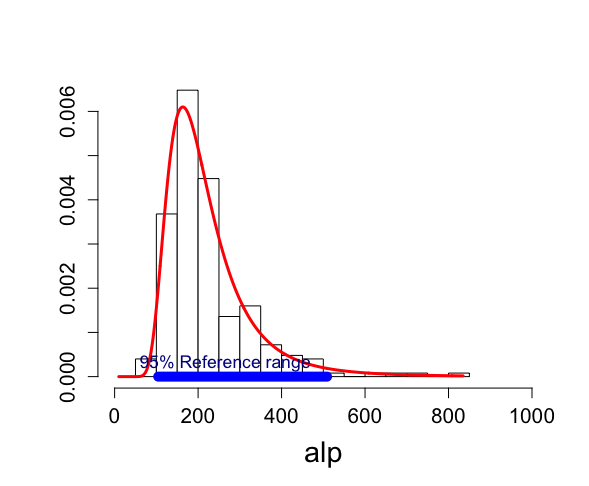
将来の観測値の分布はt249(7.11, 1.37)分布となる。したがって、yの95%正常範囲は[4.41,9.80]であり、alpの95%正常範囲は[104.1, 513.2]となる。
|
1 2 3 4 5 6 7 8 9 10 |
> # PPD > > sdppd <- sdtalp*sqrt(1+1/ntalp) > ppd.unl <- mtalp-qt(0.975,ntalp-1)*sdppd > ppd.upl <- mtalp+qt(0.975,ntalp-1)*sdppd > ppd.unl;ppd.upl;100^2/ppd.unl^2;100^2/ppd.upl^2 [1] 4.414255 [1] 9.803192 [1] 513.1982 [1] 104.0555 |
次に、後ろ向きの事前研究のデータalpのデータのalkfos[artikel==1]の65個のデータを使う。
共役事前分布はN-Inv-χ^2(5.25, 65, 64, 2.76)
事後分布はN-Inv-χ^2(6.72, 315, 314, 2.61)
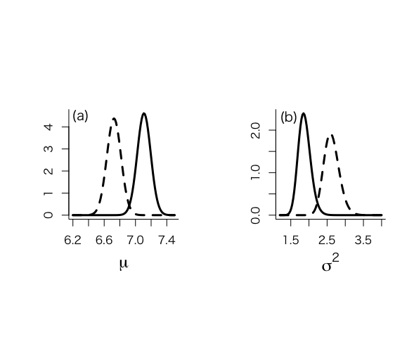
事後平均6.72は、事前平均5.25と標本平均7.11の重み付き平均である。μの事後分散は0.0083であり、以前の無情報事前分布から求めた事後分散0.0075より大きい。
μの95%信用区間は[6.54, 6.90]
σ^2の事後平均は2.62で、事後分散は0.044、95%信用区間は[2.24, 3.07]で、95%HPD区間[2.23, 3.04]
将来の観測値の分布はt314(6.72, 1.62)分布であり、yの95%信用区間は[3.54, 9.91]で、対応するalp 95%正常範囲は[101.9, 796.7]である。
|
1 2 3 4 5 6 7 8 9 10 11 12 13 14 15 16 17 18 19 20 21 22 23 24 25 26 27 28 29 30 31 32 33 34 35 36 37 38 39 40 41 42 43 44 45 46 47 48 49 50 51 52 53 54 55 56 57 58 59 60 61 62 63 64 65 66 67 68 69 70 71 72 73 74 75 76 77 78 79 80 81 82 83 84 85 86 87 88 89 90 91 92 93 94 95 96 97 98 99 100 101 102 103 104 105 106 107 108 109 110 111 112 113 114 115 116 117 118 119 120 121 122 123 124 125 126 127 128 129 130 131 132 133 134 135 136 137 138 139 140 141 142 143 144 145 146 147 148 149 150 151 152 153 154 155 156 157 158 159 160 161 162 163 164 165 166 167 168 169 170 171 172 173 174 175 176 177 178 179 180 181 182 183 184 185 186 187 188 189 190 191 192 193 194 195 196 197 198 199 200 201 202 203 204 205 206 207 208 209 210 211 212 213 214 215 216 217 218 219 220 221 222 223 224 225 226 227 228 |
> objects(2) [1] "alkfos" "artikel" > > alp <- alkfos[artikel==0] > talp <- 100*alp^(-1/2) > nalp <- length(alp) > > mtalp <- mean(talp) > vartalp <- var(talp) > sdtalp <- sqrt(var(talp)) > ntalp <- length(talp) > > mtalp;sdtalp [1] 7.108724 [1] 1.365344 > > par(mfrow=c(1,1)) > par(pty="m") > par(mar=c(5,5,4,2)+0.1) > > > # historical data calculate Ninvchイ > > par(mfrow=c(1,1)) > par(pty="m") > par(mar=c(5,5,4,2)+0.1) > > alphis <- alkfos[artikel==1] > talp0 <- 100*alphis^(-1/2) > > mtalp0 <- mean(talp0) > vartalp0 <- var(talp0) > sdtalp0 <- sqrt(var(talp0)) > ntalp0 <- length(talp0) > > mtalp0;sdtalp0;ntalp0 [1] 5.24849 [1] 1.65845 [1] 65 > > hist(talp0,xlab="100/sqrt(ALP)",nclas=30,col="light blue", + cex.lab=1.8,cex.axis=1.3,prob=T,main="") > > # prior values > > mu0 <- mtalp0 > kappa0 <- ntalp0 > nu0 <- ntalp0-1 > tau20 <- vartalp0 > > # sample values > > alp <- alkfos[artikel==0] > talp <- 100*alp^(-1/2) > > mtalp <- mean(talp) > vartalp <- var(talp) > sdtalp <- sqrt(var(talp)) > ntalp <- length(talp) > > > #posterior values > > mubar <- (kappa0*mu0+ntalp*mtalp)/(kappa0+ntalp) > kappabar <- kappa0+ntalp > nubar <- nu0 + ntalp > taubarp1 <- nu0*tau20 > taubarp2 <- (ntalp-1)*vartalp > taubarp3 <- (mtalp-mu0)^2*kappa0*ntalp/(kappa0+ntalp) > taubar2 <- (taubarp1+taubarp2+taubarp3)/nubar > > mu0;kappa0;nu0;tau20 [1] 5.24849 [1] 65 [1] 64 [1] 2.750455 > mtalp;vartalp [1] 7.108724 [1] 1.864165 > mubar;kappabar;nubar;taubar2;sqrt(taubar2) [1] 6.724866 [1] 315 [1] 314 [1] 2.607396 [1] 1.614743 > > # marginal posterior distribution of MEAN & SIGMAイ > # Figure 4.2 > > > unl.mu <- 6.2 > upl.mu <- 7.5 > > unl.sigma2 <- 1.2 > upl.sigma2 <- 4 > > nmu <- 100 > nsigma2 <- 100 > > # values using ni prior > > mu <- seq(unl.mu,upl.mu,length=nmu) > mus <- (mu-mtalp)/(sdtalp/sqrt(ntalp)) > pmu <- dt(mus,ntalp-1)*sqrt(ntalp)/sdtalp > sigma2 <- seq(unl.sigma2,upl.sigma2,length=nsigma2) > sigma2s <- (ntalp-1)*vartalp/sigma2 > psigma2 <- dchisq(sigma2s,ntalp-1)*(ntalp-1)*vartalp/(sigma2^2) > > # values from inf prior > > mub <- seq(unl.mu,upl.mu,length=nmu) > musb <- (mub-mubar)/(sqrt(taubar2)/sqrt(kappabar)) > pmub <- dt(musb,nubar)*sqrt(kappabar)/sqrt(taubar2) > sigma2b <- seq(unl.sigma2,upl.sigma2,length=nsigma2) > sigma2sb <- nubar*taubar2/sigma2b > psigma2b <- dchisq(sigma2sb,nubar)*nubar*taubar2/(sigma2b^2) > > par(mfrow=c(1,2)) > par(pty="s") > > plot(mub,pmub,type="n",xlab=expression(paste(mu)),ylab="", + ylim=c(0,max(pmu,pmub)),bty="l",main="",cex.lab=1.5) > lines(mu,pmu,lwd=3,lty=1) > lines(mub,pmub,lwd=3,,lty="dashed") > text(6.3,4.5,"(a)",cex=1.2) > > plot(sigma2b,psigma2b,type="n",xlab=expression(paste(sigma^{2})), + ylab="",ylim=c(0,max(psigma2,psigma2b)),bty="l",main="",cex.lab=1.5) > lines(sigma2,psigma2,lwd=3,lty=1) > lines(sigma2b,psigma2b,lwd=3,lty="dashed") > text(1.45,2.3,"(b)",cex=1.2) > > > # summary statistics from inf prior > > # for mu > > mupostmean <- mubar > mupostvar <- nubar*taubar2/(kappabar*(nubar-2)) > mu.post.unl <- mubar - qt(0.975,nubar)*sqrt(taubar2)/sqrt(kappabar) > mu.post.upl <- mubar + qt(0.975,nubar)*sqrt(taubar2)/sqrt(kappabar) > mupostmean;mupostvar;mu.post.unl;mu.post.upl [1] 6.724866 [1] 0.008330509 [1] 6.545857 [1] 6.903874 > > # for sigma^2 > > sigma2postmean <- taubar2*(nubar)/(nubar-2) > sigma2postmode <- taubar2*(nubar)/(nubar+2) > sigma2postmedian <- taubar2*(nubar)/qchisq(0.5,nubar) > sigma2postvar <- taubar2^2*2*(nubar)^2/((nubar-2)^2*(nubar-4)) > sigma2.post.unl <- (nubar)*taubar2/qchisq(0.975,nubar) > sigma2.post.upl <- (nubar)*taubar2/qchisq(0.025,nubar) > sigma2postmean;sigma2postmode;sigma2postmedian;sigma2postvar;sigma2.post.unl;sigma2.post.upl [1] 2.62411 [1] 2.590894 [1] 2.612942 [1] 0.04442552 [1] 2.243182 [1] 3.068626 > > > #function to calculate hpd for sigmaイ > > unl.sigma2 <- 2 > upl.sigma2 <- 3.5 > nsigma2 <- 300 > sigma2 <- seq(unl.sigma2,upl.sigma2,length=nsigma2) > sigma2s <- (nubar)*taubar2/sigma2 > psigma2 <- dchisq(sigma2s,nubar)*(nubar)*taubar2/(sigma2^2) > > a <- 1 > #h <- 20 > min <- 1 > max <- 1 > minimum <- 9999 > eps <- 0.001 > > for (a in 1:(nsigma2-1)){ + begin <- sigma2[a] + for (h in (a+1):nsigma2){ + #print(a);print(h) + end <- sigma2[h] + diffunction <- abs(psigma2[a]-psigma2[h]) + cumprobbegin <- pchisq(taubar2*(nubar)/sigma2[a], nubar) + cumprobend <- pchisq(taubar2*(nubar)/sigma2[h], nubar) + difcum <- cumprobbegin-cumprobend + if((abs(difcum-0.95) < eps) && (diffunction < minimum)) {minimum <- diffunction; min <- a; max <- h} + } + } > > min;max;minimum [1] 46 [1] 209 [1] 0.006462411 > sigma2[min];sigma2[max] [1] 2.225753 [1] 3.043478 > > par(mfrow=c(1,1)) > par(pty="m") > > plot(sigma2,psigma2,type="n",xlab=expression(paste(sigma^{2})), + ylab="Posterior",ylim=c(0,max(psigma2)),bty="l",main="",cex.lab=1.5, + cex.axis=1.2) > lines(sigma2,psigma2,lwd=3,col="dark red") > segments(sigma2[min],0,sigma2[min],psigma2[min]) > segments(sigma2[max],0,sigma2[max],psigma2[max]) > segments(sigma2[min],0,sigma2[max],0,col="dark blue",lwd=3) > text(2.6,0.15,"95% HPD interval",col="dark blue",cex=1.4) > > > # PPD > > sdppd <- sqrt(taubar2)*sqrt(1+1/kappabar) > ppd.unl <- mubar-qt(0.975,nubar)*sdppd > ppd.upl <- mubar+qt(0.975,nubar)*sdppd > ppd.unl;ppd.upl;100^2/ppd.unl^2;100^2/ppd.upl^2 [1] 3.542742 [1] 9.90699 [1] 796.7479 [1] 101.8865 > mubar;nubar;sdppd [1] 6.724866 [1] 314 [1] 1.617304 |

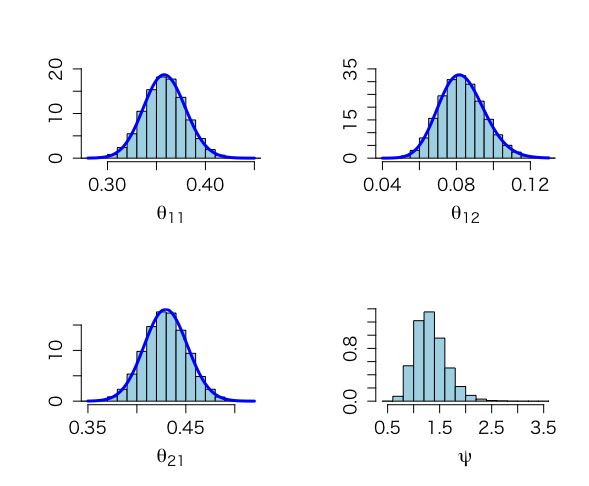
4.4 多変量分布
青年調査:喫煙と飲酒の関連
|
1 2 3 4 5 6 7 8 9 10 11 12 13 14 15 16 17 18 19 20 21 22 23 24 25 26 27 28 29 30 31 32 33 34 35 36 37 38 39 40 41 42 43 44 45 46 47 48 49 50 51 52 53 54 55 56 57 58 59 60 61 62 63 64 65 66 67 68 69 70 71 72 73 74 75 76 77 78 79 80 81 82 83 84 85 86 87 88 89 90 91 92 93 94 95 96 97 98 99 100 101 102 103 104 105 106 107 108 109 110 111 112 113 114 115 116 117 118 119 120 121 |
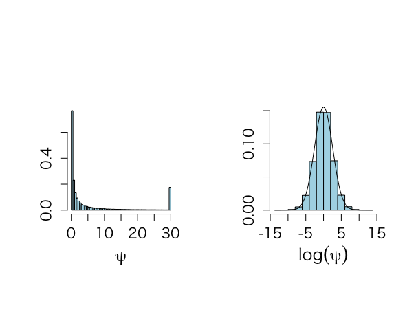
x <- c(180,41,216,64) or <- (x[1]*x[4])/(x[2]*x[3]) lor <- log(or) varlor <- 1/x[1] + 1/x[2] +1/x[3] +1/x[4] sdlor <- sqrt(varlor) unlor <- lor - 1.96*sdlor uplor <- lor + 1.96*sdlor eunlor <- exp(unlor) euplor <- exp(uplor) eunlor;euplor alpha11 <- 1+x[1] alpha12 <- 1+x[2] alpha21 <- 1+x[3] alpha22 <- 1+x[4] salpha <- alpha11+alpha12+alpha21+alpha22 set.seed(777) N <- 100000 w11 <- rgamma(N,shape=alpha11,rate=1) w12 <- rgamma(N,shape=alpha12,rate=1) w21 <- rgamma(N,shape=alpha21,rate=1) w22 <- rgamma(N,shape=alpha22,rate=1) t <- w11+w12+w21+w22 z11 <- w11/t z12 <- w12/t z21 <- w21/t z22 <- w22/t par(mfrow=c(2,2)) par(pty="m") hist(z11,prob=T,xlim=c(0.28,0.45),ylim=c(0,20),col="light blue", xlab=expression(paste(theta[11])),cex.lab=1.5,ylab="",main="", cex.axis=1.3) zgrid <- seq(0.28,0.45,0.001) lines(zgrid,dbeta(zgrid,alpha11,salpha-alpha11),lwd=3,col="blue") hist(z12,prob=T,xlim=c(0.04,0.13),ylim=c(0,35),col="light blue", xlab=expression(paste(theta[12])),cex.lab=1.5,ylab="",main="", cex.axis=1.3) zgrid <- seq(0.04,0.13,0.001) lines(zgrid,dbeta(zgrid,alpha12,salpha-alpha12),lwd=3,col="blue") hist(z21,prob=T,xlim=c(0.35,0.52),col="light blue", xlab=expression(paste(theta[21])),cex.lab=1.5,ylab="",main="", cex.axis=1.3) zgrid <- seq(0.35,0.52,0.001) lines(zgrid,dbeta(zgrid,alpha21,salpha-alpha21),lwd=3,col="blue") #hist(z22,prob=T,xlim=c(0.08,0.18), # xlab=expression(paste(theta[22])),cex.lab=1.4,ylab="",main="") #zgrid <- seq(0.08,0.18,0.001) #lines(zgrid,dbeta(zgrid,alpha22,salpha-alpha22),lwd=3,col="blue") psi <- (z11*z22)/(z12*z21) lpsi <- log(psi) hist(psi,xlab=expression(paste(psi)),prob=T,col="light blue", cex.lab=1.5,ylab="",main="", cex.axis=1.3) q <- quantile(lpsi,c(0.025,0.975)) meanq <- mean(q) q;meanq exp(q);exp(meanq) # exploring the non-informative Dirichlet prior # not in book alpha11 <- 1 alpha12 <- 1 alpha21 <- 1 alpha22 <- 1 salpha <- alpha11+alpha12+alpha21+alpha22 set.seed(777) N <- 100000 w11 <- rgamma(N,shape=alpha11,rate=1) w12 <- rgamma(N,shape=alpha12,rate=1) w21 <- rgamma(N,shape=alpha21,rate=1) w22 <- rgamma(N,shape=alpha22,rate=1) t <- w11+w12+w21+w22 z11 <- w11/t z12 <- w12/t z21 <- w21/t z22 <- w22/t psi <- (z11*z22)/(z12*z21) lpsi <- log(psi) summary(psi) mlpsi <- mean(lpsi) sdlpsi <- sqrt(var(lpsi)) max(psi) mlpsi;sdlpsi gridlpsi <- seq(min(lpsi),max(lpsi),0.1) par(mfrow=c(1,2)) par(pty="s") hist(pmin(psi,30),xlab=expression(paste(psi)),prob=T,col="light blue",xlim=c(0,30), cex.lab=1.5,ylab="",main="", cex.axis=1.3,nclas=50) hist(lpsi,xlab=expression(paste(log(psi))),prob=T,col="light blue", cex.lab=1.5,ylab="",main="", cex.axis=1.3,ylim=c(0,0.15)) lines(gridlpsi,dnorm(gridlpsi,mlpsi,sdlpsi)) |
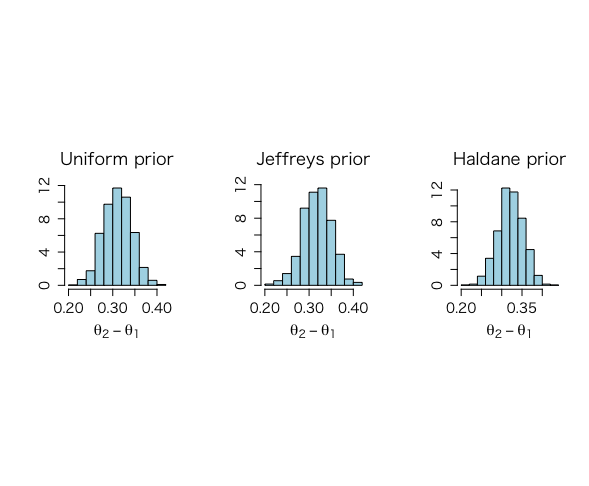
Kaldor’s et al. のケース・コントロール研究:例?.9の再解析
|
1 2 3 4 5 6 7 8 9 10 11 12 13 14 15 16 17 18 19 20 21 22 23 24 25 26 27 28 29 30 31 32 33 34 35 36 37 38 39 40 41 42 43 44 45 46 47 48 49 50 51 52 53 54 55 56 57 58 59 60 61 62 63 64 65 66 67 68 69 70 71 72 73 74 |
# Kaldor case-control study xcontrol <- c(251,160) xcase <- c(138,11) set.seed(777) par(mfrow=c(1,3)) par(pty="s") par(mar=c(5,5,4,2)+0.1) # uniform prior a0 <- 1 b0 <- 1 c0 <- 1 d0 <- 1 a <- 251 b <- 160 c <- 138 d <- 11 N <- 1000 theta1 <- rbeta(N,a0+a,b0+b) theta2 <- rbeta(N,c0+c,d0+d) dtheta <- theta2-theta1 mean(dtheta) quantile(dtheta,c(0.025,0.975)) hist(dtheta,prob=T,col="light blue", xlab=expression(theta[2]-theta[1]),cex.lab=1.5,ylab="",main="Uniform prior", cex.axis=1.3,cex.main=1.6) # Jeffreys prior a0 <- -1/2 b0 <- -1/2 c0 <- -1/2 d0 <- -1/2 theta1 <- rbeta(N,a0+a,b0+b) theta2 <- rbeta(N,c0+c,d0+d) dtheta <- theta2-theta1 mean(dtheta) quantile(dtheta,c(0.025,0.975)) hist(dtheta,prob=T,col="light blue", xlab=expression(theta[2]-theta[1]),cex.lab=1.5,ylab="",main="Jeffreys prior", cex.axis=1.3,cex.main=1.6) # Haldane prior a0 <- -1 b0 <- -1 c0 <- -1 d0 <- -1 theta1 <- rbeta(N,a0+a,b0+b) theta2 <- rbeta(N,c0+c,d0+d) dtheta <- theta2-theta1 mean(dtheta) quantile(dtheta,c(0.025,0.975)) hist(dtheta,prob=T,col="light blue", xlab=expression(theta[2]-theta[1]),cex.lab=1.5,ylab="",main="Haldane prior", cex.axis=1.3,cex.main=1.6) |
4.5 ベイズ推測の頻度論的な性質
|
1 2 3 4 5 6 7 8 9 10 11 12 13 14 15 16 17 18 19 20 21 22 23 24 25 26 27 28 29 30 31 32 33 34 35 36 37 38 39 40 41 42 43 44 45 46 47 48 49 50 51 52 53 54 55 56 57 58 59 60 61 62 63 64 65 66 67 68 69 70 71 72 73 74 75 76 77 78 79 80 81 82 83 84 85 86 87 88 89 90 91 92 93 94 95 96 97 98 99 100 101 102 103 104 105 106 107 108 109 110 111 112 113 114 115 116 117 118 119 120 121 122 123 124 125 126 |
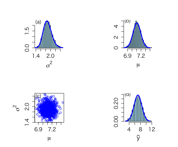
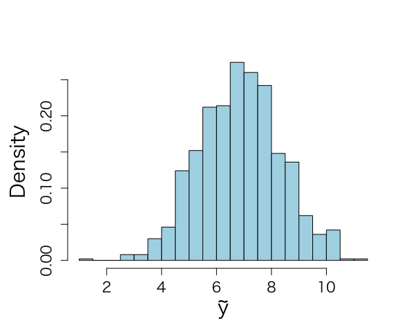
# SAMPLING FROM NONINFORMATIVE PRIOR attach(ALP) objects(2) alp <- alkfos[artikel==0] talp <- 100*alp^(-1/2) mtalp <- mean(talp) vartalp <- var(talp) sdtalp <- sqrt(var(talp)) ntalp <- length(talp) # sample from sigma then from mu given sigma (1000 times), make use of theoretical results # Figure 4.3 set.seed(777) unl.mu <- 6.8 upl.mu <- 7.4 unl.sigma2 <- 1.2 upl.sigma2 <- 2.5 nmu <- 50 nsigma2 <- 50 ntilde <- 50 mu <- seq(unl.mu,upl.mu,length=nmu) mus <- (mu-mtalp)/(sdtalp/sqrt(ntalp)) pmu <- dt(mus,ntalp-1)*sqrt(ntalp)/sdtalp sigma2 <- seq(unl.sigma2,upl.sigma2,length=nsigma2) sigma2s <- (ntalp-1)*vartalp/sigma2 psigma2 <- dchisq(sigma2s,ntalp-1)*(ntalp-1)*vartalp/(sigma2^2) par(mfrow=c(2,2)) par(pty="s") par(mar=c(5,4,4,2)+0.1) nsimul <- 1000 #posterior distribution of sigma^2 phi.u <- rchisq(nsimul,ntalp-1) theta.u <- 1/phi.u sigma.u <- sqrt((ntalp-1)*vartalp*theta.u) # posterior summary statistics meansamplesigma2 <- mean(sigma.u^2) sdsamplesigma2 <- sqrt(var(sigma.u^2)) unl.conf <- meansamplesigma2 -1.96*sdsamplesigma2/sqrt(nsimul) upl.conf <- meansamplesigma2 +1.96*sdsamplesigma2/sqrt(nsimul) meansamplesigma2;sdsamplesigma2;unl.conf;upl.conf quantile(sigma.u^2, c(.025,.975)) hist(sigma.u^2,xlab=expression(sigma^{2}), ylab="", main="", nclas=30,prob=T,cex.lab=1.5,col="light blue", cex.axis=1.3) lines(sigma2,psigma2,lwd=3,lty=1,col="blue") text(1.5,2.3,"(a)",cex=1.2) #conditional posterior distribution of mu given sigma^2 mucond1.u <- rnorm(nsimul,mtalp,sdtalp/sqrt(ntalp)) mucond2.u <- rnorm(nsimul,mtalp,2.5/sqrt(ntalp)) #hist(mucond1.u,xlab="MU values, given SIGMA = SAMPLE VARIANCE", #ylab="HISTOGRAM",main="(b)",nclas=30,prob=T) #hist(mucond2.u,xlab="Posterior sampled MU values,given SIGMA = 2.5",nclas=30,prob=T) #marginal posterior distribution of mu given sigma^2 mu.u <- rnorm(nsimul,mtalp,sigma.u/sqrt(ntalp)) # posterior summary statistics meansamplemu <- mean(mu.u) sdsamplemu <- sqrt(var(mu.u)) unl.conf <- meansamplemu -1.96*sdsamplemu/sqrt(nsimul) upl.conf <- meansamplemu +1.96*sdsamplemu/sqrt(nsimul) meansamplemu;sdsamplemu;unl.conf;upl.conf quantile(mu.u, c(.025,.975)) hist(mu.u,xlab=expression(paste(mu)),ylab="",main="", nclas=30,prob=T,cex.lab=1.5,col="light blue", cex.axis=1.3) lines(mu,pmu,lwd=3,lty=1,col="blue") text(6.9,5,"(b)",cex=1.2) #joint posterior distribution of mu and sigma^2 plot(mu.u,sigma.u^2,xlab=expression(paste(mu)),ylab=expression(paste(sigma^{2})), main="",cex.lab=1.5,col="blue", cex.axis=1.3) text(6.9,2.4,"(c)",cex=1.2) #sample from ppd future.u <- rnorm(nsimul,mu.u,sigma.u) hist(future.u,xlab=expression(tilde(y)),nclas=30,prob=T,main="", cex.lab=1.5,ylab="",ylim=c(0,0.3),col="light blue", cex.axis=1.3) text(3.5,0.3,"(d)",cex=1.2) py.unl <- mtalp -qt(0.999,ntalp-1)*sdtalp*sqrt(1+1/ntalp) py.upl <- mtalp +qt(0.999,ntalp-1)*sdtalp*sqrt(1+1/ntalp) tildey <- seq(py.unl,py.upl,length=ntilde) tildeys <- (tildey-mtalp)/(sdtalp/sqrt(1+1/ntalp)) ptildey <- dt(tildeys,ntalp-1)*sqrt(1+1/ntalp)/sdtalp lines(tildey,ptildey,lwd=3,lty=1,col="blue") |
4.6 事後分布からのサンプリング:合成法
|
1 2 3 4 5 6 7 8 9 10 11 12 13 14 15 16 17 18 19 20 21 22 23 24 25 26 27 28 29 30 31 32 33 34 35 36 37 38 39 40 41 42 43 44 45 46 47 48 49 50 51 52 53 54 55 56 57 58 59 60 61 62 63 64 65 66 67 68 69 70 71 72 73 74 75 76 77 78 79 80 81 82 83 84 85 86 87 88 89 90 91 92 93 94 95 96 97 98 99 100 101 102 103 104 105 106 107 108 109 110 111 112 113 114 115 116 117 118 119 120 121 122 123 124 125 126 127 128 129 130 131 132 133 134 135 136 137 138 139 140 141 142 143 144 145 146 147 148 149 150 151 152 153 154 155 156 157 158 159 160 161 162 163 164 165 166 167 168 169 170 171 172 173 174 175 176 177 178 179 180 181 182 183 184 185 186 187 188 189 190 191 192 193 194 195 196 197 198 199 200 201 202 203 204 205 206 207 208 209 210 211 212 213 214 215 216 217 218 219 220 221 222 223 224 225 226 227 228 229 230 231 232 233 234 235 236 237 238 239 240 241 242 243 244 245 246 247 248 249 250 251 252 253 254 255 256 |
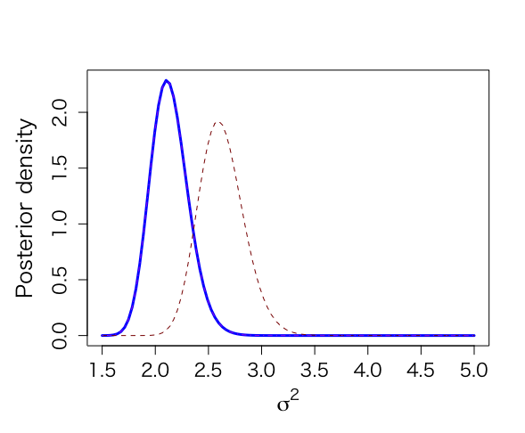
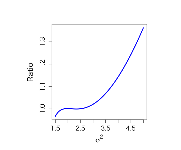
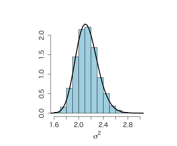
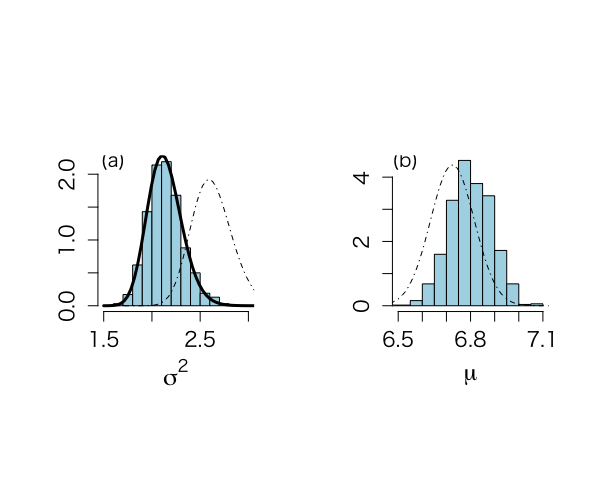
# Figure 4.4 # SAMPLING FROM PRODUCT OF INFORMATIVE PRIORS, using Method of Composition attach(ALP) objects(2) # historical data calculate Ninvchイ alphis <- alkfos[artikel==1] talp0 <- 100*alphis^(-1/2) mtalp0 <- mean(talp0) vartalp0 <- var(talp0) sdtalp0 <- sqrt(var(talp0)) ntalp0 <- length(talp0) mtalp0;sdtalp0;ntalp0 par(mfrow=c(1,1)) par(pty="m") # histogram of transformed response, graph is not included in book hist(talp0,xlab="100/sqrt(ALP)",nclas=30,col="light blue", cex.lab=1.8,cex.axis=1.3,prob=T,main="") # We use historical data to calculate prior values mu0 <- mtalp0 sigma20 <- vartalp0/ntalp0 nu0 <- ntalp0-1 tau20 <- vartalp0 kappa0 <- ntalp0 mu0;sigma20;nu0;tau20 # Data from prospective study with 250 individuals (current study) alp <- alkfos[artikel==0] talp <- 100*alp^(-1/2) mtalp <- mean(talp) vartalp <- var(talp) sdtalp <- sqrt(var(talp)) ntalp <- length(talp) mtalp;vartalp;sdtalp;ntalp # Start the sampling procedure via Method of Composition # First sample sigma^2, then mu # For sigma^2 we need a trick since posterior is known up to a constant # We use here SIR based on an approximating scale inv-chisqd distribution unl.mu <- 6.2 upl.mu <- 7.4 unl.sigma2 <- 1.5 upl.sigma2 <- 5 nmu <- 100 nsigma2 <- 100 ntilde <- 100 sigma2 <- seq(unl.sigma2,upl.sigma2,length=nsigma2) gridsize <- sigma2[2]-sigma2[1] mubar <- (mu0/sigma20+ntalp*mtalp/sigma2)/(1/sigma20+ntalp/sigma2) taubar2 <- 1/(1/sigma20+ntalp/sigma2) sigma2s <- nu0*tau20/sigma2 psigma2 <- dchisq(sigma2s,nu0)*nu0*tau20/(sigma2^2) loglastfact <- rep(0,nsigma2) for (i in 1:ntalp){ loglastfact <- loglastfact + log(dnorm(talp[i],mean=mubar,sd=sqrt(sigma2))) } loglastfact <- loglastfact - min(loglastfact) lastfact <- exp(loglastfact) psigma2bar <- sqrt(taubar2)*dnorm(mubar,mean=mu0,sd=sqrt(sigma20))*psigma2*lastfact totalarea <- sum(psigma2bar)*gridsize spsigma2bar <- psigma2bar/totalarea # Distribution from joint conjugate prior, serves as a comparison mubarj <- (kappa0*mu0+ntalp*mtalp)/(kappa0+ntalp) kappabarj <- kappa0+ntalp nubarj <- nu0 + ntalp taubarp1j <- nu0*tau20 taubarp2j <- (ntalp-1)*vartalp taubarp3j <- (mtalp-mu0)^2*kappa0*ntalp/(kappa0+ntalp) taubar2j <- (taubarp1j+taubarp2j+taubarp3j)/nubarj sigma2sj <- nubarj*taubar2j/sigma2 psigma2conjugate <- dchisq(sigma2sj,nubarj)*nubarj*taubar2j/(sigma2^2) # Approximating inv chisq distribution, to be used in SIR sampling later on moment1sigma2bar <- spsigma2bar%*%sigma2*gridsize moment2sigma2bar <- spsigma2bar%*%sigma2^2*gridsize varsigma2bar <- moment2sigma2bar-moment1sigma2bar^2 a <- moment1sigma2bar b <- varsigma2bar df <- 2*a^2/b+4 s2 <- (df-2)*a/df sigma2s <- df*s2/sigma2 psigma2approx <- dchisq(sigma2s,df)*df*s2/(sigma2^2) # Graphs not shown in book to compare # p(sigma^2| y) as given by expression (4.19) in book: spsigma2bar # Conjugate prior based on equivalent information: psigma2conjugate # Approximate scaled inverse chi^2 distribution: psigma2approx par(mar=c(5,5,4,2)+0.1) plot(sigma2,spsigma2bar,xlab=expression(sigma^{2}),ylab="Posterior density", type="n", main="",cex.lab=1.5,cex.axis=1.3) lines(sigma2,spsigma2bar,lwd=3,col="blue") lines(sigma2,psigma2conjugate,lty=2,col="dark red") lines(sigma2,psigma2approx,lty=4,col="purple") # Evaluate (4.19) with approximation par(pty="s") plot(sigma2,spsigma2bar/psigma2approx,xlab=expression(sigma^{2}), ylab="Ratio", type="n", main="",cex.lab=1.5,cex.axis=1.3) lines(sigma2,spsigma2bar/psigma2approx,lwd=3,col="blue") # Weighted resampling (SIR) method # We sample from approximating scaled inv-chisqd distribution, then resample NSIMUL <- 10000 nsimul <- 1000 set.seed(777) phi.u <- rchisq(NSIMUL,df) theta.u <- 1/phi.u sigma2.1 <- df*s2*theta.u nsigma2 <- 100 sigma2 <- seq(unl.sigma2,upl.sigma2,length=nsigma2) sigma2s <- df*s2/sigma2 psigma2approx <- dchisq(sigma2s,df)*df*s2/(sigma2^2) # Histogram of sample of sigma^2 from approximate scaled inverse-chi^2 distribution hist(sigma2.1,prob=T,xlab=expression(sigma^{2}), ylab="",main="",cex.lab=1.5,col="light blue", cex.axis=1.3) lines(sigma2,psigma2approx,lwd=3) mubar.u <- (mu0/sigma20+ntalp*mtalp/sigma2.1)/(1/sigma20+ntalp/sigma2.1) taubar2.u <- 1/(1/sigma20+ntalp/sigma2.1) sigma2s.u <- nu0*tau20/sigma2.1 psigma2.u <- dchisq(sigma2s.u,nu0)*nu0*tau20/(sigma2.1^2) loglastfact.u <- rep(0, NSIMUL) for (i in 1:ntalp){ loglastfact.u <- loglastfact.u + log(dnorm(talp[i],mean=mubar.u,sd=sqrt(sigma2.1))) } loglastfact.u <- loglastfact.u - min(loglastfact.u) lastfact.u <- exp(loglastfact.u) post2 <- sqrt(taubar2.u)*dnorm(mubar.u,mean=mu0,sd=sqrt(sigma20))*psigma2.u*lastfact.u sigma2sappr.u <- df*s2/sigma2.1 post1 <- dchisq(sigma2sappr.u,df)*df*s2/(sigma2.1^2) v <- post2/post1 w <- v/sum(v) # Now resample sigma2.2 <- sample(sigma2.1, size=nsimul, replace=F, prob=w) # Figure 4.4, obtained from Method of Composition par(mfrow=c(1,2)) par(pty="s") hist(sigma2.2,prob=T,xlab=expression(sigma^{2}), ylab="",main="",cex.lab=1.5,col="light blue",ylim=c(0,2.2),xlim=c(1.5,3), cex.axis=1.3) lines(sigma2,spsigma2bar,lwd=3) lines(sigma2,psigma2conjugate,lty=4) text(1.6,2.2,"(a)",cex=1.2) pmean <- mean(sigma2.2) pmedian <- median(sigma2.2) pvar <- var(sigma2.2) quantile(sigma2.2,c(0.025,0.975)) unl.conf <- pmean -1.96*sqrt(pvar)/sqrt(length(sigma2.2)) upl.conf <- pmean +1.96*sqrt(pvar)/sqrt(length(sigma2.2)) pmean;pmedian;pvar;unl.conf;upl.conf #Now sample mu mubar.2 <- (mu0/sigma20+ntalp*mtalp/sigma2.2)/(1/sigma20+ntalp/sigma2.2) sigma2bar.2 <- 1/(1/sigma20+ntalp/sigma2.2) mu.2 <- rnorm(nsimul,mean=mubar.2, sd=sqrt(sigma2bar.2)) hist(mu.2,xlab=expression(mu),prob=T, ylab="",main="",cex.lab=1.5,col="light blue",ylim=c(0,4.5),xlim=c(6.5,7.1), cex.axis=1.3) text(6.53,4.5,"(b)",cex=1.2) # Compare with posterior obtained from conjugate muj <- seq(unl.mu,upl.mu,length=nmu) musj <- (muj-mubarj)/(sqrt(taubar2j)/sqrt(kappabarj)) pmuj <- dt(musj,nubarj)*sqrt(kappabarj)/sqrt(taubar2j) lines(muj,pmuj,lty=4) pmean <- mean(mu.2) pmedian <- median(mu.2) pvar <- var(mu.2) quantile(mu.2,c(0.025,0.975)) unl.conf <- pmean -1.96*sqrt(pvar)/sqrt(length(mu.2)) upl.conf <- pmean +1.96*sqrt(pvar)/sqrt(length(mu.2)) pmean;pmedian;pvar;unl.conf;upl.conf # Sample from ppd, figure not shown in book par(mfrow=c(1,1)) par(pty="m") future.u <- rnorm(nsimul,mu.2,sqrt(sigma2.2)) hist(future.u,xlab=expression(tilde(y)),nclas=30,col="light blue", cex.lab=1.8,cex.axis=1.3,prob=T,main="") mean(future.u) qfuturey <- quantile(future.u,c(0.025,0.975)) qfutureALT <- 100^2/qfuturey^2 qfuturey;qfutureALT |
4.7 ベイズ流線形回帰モデル
|
1 2 3 4 5 6 7 8 9 10 11 12 13 14 15 16 17 18 19 20 21 22 23 24 25 26 27 28 29 30 31 32 33 34 35 36 37 38 39 40 41 42 43 44 45 46 47 48 49 50 51 52 53 54 55 56 57 58 59 60 61 62 63 64 65 66 67 68 69 70 71 72 73 74 75 76 77 78 |
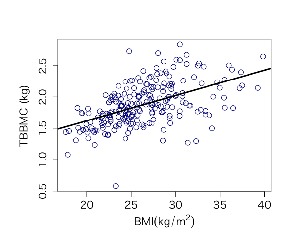
> osteop =read.delim("osteop.txt", header=TRUE) > library(mvtnorm) > > attach(osteop) > > objects(2) [1] "AGE" "BMI" "TBBMC" > > > bmi <- BMI > tbbmc <- TBBMC > age <- AGE > > x <- bmi[!is.na(tbbmc)] > y <- tbbmc[!is.na(tbbmc)] > z <- age[!is.na(tbbmc)] > > #output data set > > summary(x) Min. 1st Qu. Median Mean 3rd Qu. Max. 17.61 23.24 25.83 26.35 28.99 39.84 > summary(y) Min. 1st Qu. Median Mean 3rd Qu. Max. 0.579 1.661 1.847 1.877 2.071 2.837 > summary(lm(y ~x)) Call: lm(formula = y ~ x) Residuals: Min 1Q Median 3Q Max -1.17225 -0.18563 -0.00723 0.19234 0.91579 Coefficients: Estimate Std. Error t value Pr(>|t|) (Intercept) 0.812856 0.115034 7.066 1.85e-11 *** x 0.040390 0.004308 9.376 < 2e-16 *** --- Signif. codes: 0 ‘***’ 0.001 ‘**’ 0.01 ‘*’ 0.05 ‘.’ 0.1 ‘ ’ 1 Residual standard error: 0.2869 on 232 degrees of freedom Multiple R-squared: 0.2748, Adjusted R-squared: 0.2717 F-statistic: 87.91 on 1 and 232 DF, p-value: < 2.2e-16 > > attributes(summary(lm(y ~x))) $names [1] "call" "terms" "residuals" "coefficients" "aliased" [6] "sigma" "df" "r.squared" "adj.r.squared" "fstatistic" [11] "cov.unscaled" $class [1] "summary.lm" > attributes(lm(y ~x))$coefficients NULL > lm(y ~x)$coefficients (Intercept) x 0.81285570 0.04038977 > > summary(lm(y ~x))$coefficients Estimate Std. Error t value Pr(>|t|) (Intercept) 0.81285570 0.115033708 7.066239 1.846215e-11 x 0.04038977 0.004307706 9.376167 6.418537e-18 > > # Figure 4.5 > > par(mfrow=c(1,1)) > par(pty="m") > > par(mar = c(5,6,4,2)+0.1) > plot(x,y,xlab=expression(paste("BMI"(kg/m^{2}))),ylab="TBBMC (kg)", + type="n",xlim=c(min(x),max(x)),cex.lab=1.3,cex=1.2,cex.axis=1.3) > points(x,y,col="dark blue",cex=1.4) > abline(lm(y ~x),lwd=3) > > |
4.8 ベイズ流一般化線形モデル
|
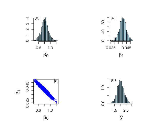
1 2 3 4 5 6 7 8 9 10 11 12 13 14 15 16 17 18 19 20 21 22 23 24 25 26 27 28 29 30 31 32 33 34 35 36 37 38 39 40 41 42 43 44 45 46 47 48 49 50 51 52 53 54 55 56 57 58 59 60 61 62 63 64 65 66 67 68 69 70 71 72 73 74 75 76 77 78 79 80 81 82 83 84 85 86 87 88 89 90 91 92 93 94 95 96 97 98 99 100 101 102 103 104 105 106 107 108 109 110 111 112 113 114 115 116 117 118 119 120 121 122 123 124 125 126 |
objects(2) x <- bmi[!is.na(tbbmc)] y <- tbbmc[!is.na(tbbmc)] z <- age[!is.na(tbbmc)] # Figure 4.6 # APPLY METHOD OF COMPOSITION mx <- mean(x) n <- length(x) my <- mean(y) s <- summary(lm(y ~x))$sigma s2 <- s^2 df <- n-2 ones <- rep(1,n) X <- matrix(cbind(ones,x),ncol=2) covpartial <- solve(t(X)%*%X) covmat <- s2*solve(t(X)%*%X) mbeta <- lm(y ~x)$coefficients mbeta # sample from sigma then from beta given sigma (1000 times), make use of theoretical results set.seed(777) par(mfrow=c(2,2)) par(pty="s") nsimul <- 1000 #posterior distribution of sigma^2 phi.u <- rchisq(nsimul,n-2) theta.u <- 1/phi.u sigma2.u <- (n-2)*s2*theta.u # posterior summary statistics meansamplesigma2 <- mean(sigma2.u) sdsamplesigma2 <- sqrt(var(sigma2.u)) unl.conf <- meansamplesigma2 -1.96*sdsamplesigma2/sqrt(nsimul) upl.conf <- meansamplesigma2 +1.96*sdsamplesigma2/sqrt(nsimul) meansamplesigma2;sdsamplesigma2;unl.conf;upl.conf quantile(sigma2.u, c(.025,.975)) # NOT IN GRAPH !!! #hist(sigma2.u,xlab="SIGMA^2",ylab="HISTOGRAM", nclas=30,prob=T) #marginal posterior distribution of mu given sigma^2 rbeta.u <- matrix(rep(NA,2*nsimul),ncol=2) covpartial <- solve(t(X)%*%X) isimul <- 1 for (isimul in 1:nsimul){ rbeta.u[isimul,] <- rmvnorm(1,mean=mbeta,sigma=sigma2.u[isimul]*covpartial) } # posterior summary statistics meanbeta <- rep(NA,2) sdbeta <- rep(NA,2) unl.conf <- rep(NA,2) upl.conf <- rep(NA,2) meanbeta[1] <- mean(rbeta.u[,1]) meanbeta[2] <- mean(rbeta.u[,2]) sdbeta[1] <- sqrt(var(rbeta.u[,1])) sdbeta[2] <- sqrt(var(rbeta.u[,2])) unl.conf[1] <- meanbeta[1] -1.96*sdbeta[1]/sqrt(nsimul) upl.conf[1] <- meanbeta[1] +1.96*sdbeta[1]/sqrt(nsimul) unl.conf[2] <- meanbeta[2] -1.96*sdbeta[2]/sqrt(nsimul) upl.conf[2] <- meanbeta[2] +1.96*sdbeta[2]/sqrt(nsimul) meanbeta sdbeta unl.conf[1];upl.conf[1] unl.conf[2];upl.conf[2] quantile(rbeta.u[,1], c(.025,.975)) quantile(rbeta.u[,2], c(.025,.975)) hist(rbeta.u[,1],xlab=expression(paste(beta[0])), ylab="",main="",nclas=30,prob=T,cex.lab=1.5,col="light blue") text(0.55,4,"(a)",cex=1.2) hist(rbeta.u[,2],xlab=expression(paste(beta[1])), ylab="",main="",nclas=30,prob=T,cex.lab=1.5,col="light blue") text(0.028,100,"(b)",cex=1.2) #joint posterior distribution of beta_0 and beta_1 plot(rbeta.u[,1], rbeta.u[,2],xlab=expression(paste(beta[0])), ylab=expression(paste(beta[1])), main="",type="n",cex.lab=1.5,bty="o") points(rbeta.u[,1], rbeta.u[,2],col="blue",cex=1.3) text(1.2,0.052,"(c)",cex=1.2) #sample from ppd xtilde <- as.vector(c(1,30)) varxtilde <- xtilde%*%covpartial%*%xtilde future.u <- rep(NA,nsimul) isimul <- 1 for (isimul in 1:nsimul){ meanfuture <- xtilde%*%rbeta.u[isimul,] sdfuture <- sqrt(sigma2.u[isimul]*(1+varxtilde)) future.u[isimul] <- rnorm(1,mean=meanfuture,sd=sdfuture) } hist(future.u,xlab=expression(paste(tilde(y))),nclas=30, prob=T,main="",cex.lab=1.5,ylab="",col="light blue") text(1.4,1.5,"(d)",cex=1.2) meanytilde <- mean(future.u) sdytilde <- sqrt(var(future.u)) meanytilde;sdytilde quantile(future.u, c(.025,.975)) |