練習問題1-6
4.
a)
binomial.conf.interval<- function(y,n) { z <- qnorm(.90) phat <- y/n se <- sqrt(phat * (1 - phat)/n) return(c(phat - z * se, phat + z * se)) } b) > ?rbinom
The Binomial Distribution

Description

Density, distribution function, quantile function and random generation for the binomial distribution with parameters size and prob.

This is conventionally interpreted as the number of ‘successes’ in size trials.

Usage

dbinom(x, size, prob, log = FALSE)
pbinom(q, size, prob, lower.tail = TRUE, log.p = FALSE)
qbinom(p, size, prob, lower.tail = TRUE, log.p = FALSE)
rbinom(n, size, prob)
Arguments

x, q
vector of quantiles.
p
vector of probabilities.
n
number of observations. If length(n) > 1, the length is taken to be the number required.
size
number of trials (zero or more).
prob
probability of success on each trial.
log, log.p
logical; if TRUE, probabilities p are given as log(p).
lower.tail
logical; if TRUE (default), probabilities are P[X ? x], otherwise, P[X > x].

> y <- rbinom(1, 20, 0.5) > y
[1] 13
> y_90 <- binomial.conf.interval(y,20) > y_90
[1] 0.5133179 0.7866821

> y <- rbinom(20, 20, 0.5) > y
[1] 15 12 14 12 12 11 9 12 10 11 9 9 14 11 9 9 10 6 11 10
> y_90 <- binomial.conf.interval(y,20) > y_90
[1] 0.6259143 0.4596131 0.5686800 0.4596131 0.4596131 0.4074364 0.3074364
[8] 0.4596131 0.3567182 0.4074364 0.3074364 0.3074364 0.5686800 0.4074364
[15] 0.3074364 0.3074364 0.3567182 0.1686800 0.4074364 0.3567182 0.8740857
[22] 0.7403869 0.8313200 0.7403869 0.7403869 0.6925636 0.5925636 0.7403869
[29] 0.6432818 0.6925636 0.5925636 0.5925636 0.8313200 0.6925636 0.5925636
[36] 0.5925636 0.6432818 0.4313200 0.6925636 0.6432818

> y_90_low <- y_90[1:20] > mean(y_90_low)
[1] 0.4003744
> y_90_high <- y_90[21:40] > mean(y_90_high)
[1] 0.6796256

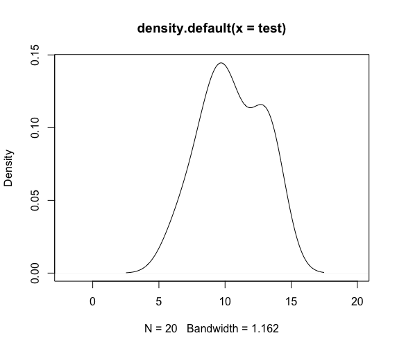
> test <- replicate(20, rbinom(1, 20, 0.5)) > test
[1] 12 11 9 7 9 10 7 8 9 15 9 12 10 13 9 12 11 11 7 11

> plot(density(test), xlim=c(-2, 20))

c)
> y <- rbinom(20, 20, 0.05) > y
[1] 0 0 0 1 0 0 1 0 2 2 1 2 1 0 0 2 2 3 0 0
> y_90 <- binomial.conf.interval(y,20) > y_90
[1] 0.00000000 0.00000000 0.00000000 -0.01245510 0.00000000 0.00000000
[7] -0.01245510 0.00000000 0.01403091 0.01403091 -0.01245510 0.01403091
[13] -0.01245510 0.00000000 0.00000000 0.01403091 0.01403091 0.04767631
[19] 0.00000000 0.00000000 0.00000000 0.00000000 0.00000000 0.11245510
[25] 0.00000000 0.00000000 0.11245510 0.00000000 0.18596909 0.18596909
[31] 0.11245510 0.18596909 0.11245510 0.00000000 0.00000000 0.18596909
[37] 0.18596909 0.25232369 0.00000000 0.00000000
> y_90_low <- y_90[1:20] > y_90_high <- y_90[21:40] > mean(y_90_low)
[1] 0.003400523
> mean(y_90_high)
[1] 0.08159948
>
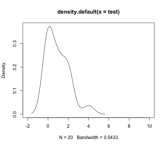
> test <- replicate(20, rbinom(1, 20, 0.05)) > test
[1] 0 1 1 2 0 0 0 0 1 0 0 2 0 0 2 2 1 1 2 4
> plot(density(test))
> plot(density(test), xlim=c(-2, 10))

5.
> test <- replicate(1000, rbinom(1, 100, 0.5)) > plot(density(test), xlim=c(-2, 100))

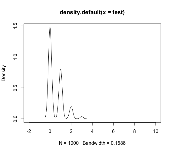
test <- replicate(1000, rbinom(1, 10, 0.05)) > plot(density(test), xlim=c(-2, 10))

sim_func <- function(n,p,m) { test <- replicate(m, rbinom(1, n, p)) y_90 <- binomial.conf.interval(test,n) plot(density(test), xlim=c(-2, m)) return(y_90) } > sim_func(20, 0,5, 20)
sim_func(20, 0, 5, 20) でエラー: 使われていない引数 (20)
> sim_func(20, 0.5, 20)
[1] 0.3567182 0.3567182 0.3074364 0.1686800 0.5686800 0.2133179 0.3074364
[8] 0.5133179 0.5133179 0.4074364 0.4596131 0.5133179 0.2596131 0.3074364
[15] 0.5133179 0.3567182 0.4074364 0.3567182 0.2596131 0.5686800 0.6432818
[22] 0.6432818 0.5925636 0.4313200 0.8313200 0.4866821 0.5925636 0.7866821
[29] 0.7866821 0.6925636 0.7403869 0.7866821 0.5403869 0.5925636 0.7866821
[36] 0.6432818 0.6925636 0.6432818 0.5403869 0.8313200