「Bayesian Computation with R」から、Ramsey&Schafer「野鳥の絶滅期間について」
まずは、LearnBayesライブラリーからbirdextinctデータを取り込む。
> library(LearnBayes)
> data(birdextinct)
> attach(birdextinct)
データ構造を確認する。以下のように平均絶滅期間(time)、つがいの平均数(nesting)、鳥のサイズ(size 大か小か)、渡り鳥かどうか(status)。
> birdextinct
species time nesting size status
1 Sparrowhawk 3.030 1.000 0 1
2 Buzzard 5.464 2.000 0 1
3 Kestrel 4.098 1.210 0 1
4 Peregrine 1.681 1.125 0 1
5 Grey_partridge 8.850 5.167 0 1
6 Quail 1.493 1.000 0 0
7 Red-legged_partridge 7.692 2.750 0 1
8 Pheasant 3.846 5.630 0 1
9 Water_rail 16.667 3.000 0 1
10 Corncrake 4.219 4.670 0 0
11 Moorhen 8.130 4.056 0 1
12 Coot 5.000 1.000 0 1
13 Lapwing 7.299 6.960 0 0
14 Golden_plover 1.000 1.670 0 0
15 Ringed_plover 27.027 5.560 0 1
16 Curlew 3.106 2.830 0 0
17 Redshank 4.000 4.375 0 0
18 Snipe 16.129 4.125 0 0
19 Stock_dove 3.484 3.670 0 1
20 Rock_dove 37.037 8.330 0 1
21 Wood_pigeon 7.299 2.750 0 1
22 Cuckoo 2.525 1.430 0 0
23 Short-eared_owl 4.132 2.000 0 1
24 Little_owl 2.000 2.750 0 1
25 Magpie 10.000 4.500 0 1
26 Jackdaw 2.667 7.120 0 1
27 Carrion_crow 4.587 4.580 0 1
28 Raven 58.824 2.350 0 1
29 Skylark 32.258 6.870 1 1
30 Swallow 2.571 3.830 1 0
31 House_martin 2.160 5.000 1 0
32 Yellow_wagtail 1.000 1.250 1 0
33 Pied_wagtail 2.967 2.270 1 1
34 Meadow_pipit 9.524 5.350 1 1
35 Wren 11.111 8.700 1 1
36 Dunnock 7.299 6.100 1 1
37 Robin 4.000 3.330 1 1
38 Stonechat 2.381 3.640 1 1
39 Wheatear 2.611 4.830 1 0
40 Blackbird 3.257 4.670 1 1
41 Song_thrush 1.701 1.700 1 1
42 Mistle_thrush 1.795 1.330 1 1
43 Grasshopper_warbler 1.198 1.000 1 0
44 Sedge_warbler 3.185 1.900 1 0
45 Whitethroat 2.273 4.420 1 0
46 Willow_warbler 1.111 1.250 1 0
47 Chiffchaff 1.000 1.000 1 0
48 Goldcrest 1.000 1.000 1 1
49 Spotted_flycatcher 1.230 1.000 1 0
50 Great_tit 6.061 2.500 1 1
51 Blue_tit 3.175 1.500 1 1
52 Yellowhammer 2.000 2.500 1 1
53 Reed_bunting 5.076 5.630 1 1
54 Chaffinch 1.934 2.370 1 1
55 Goldfinch 1.493 1.500 1 1
56 Redpoll 1.000 1.000 1 1
57 Linnet 5.102 6.500 1 1
58 House_sparrow 3.003 4.500 1 1
59 Tree_sparrow 1.898 2.170 1 1
60 Starling 41.667 11.620 1 1
61 Pied_flycatcher 1.000 1.000 1 0
62 Siskin 1.000 1.000 1 1
ここでのプロジェクトは、絶滅期間(time)を、共変量nesting, size, statusによって?明できるモデルに当てはめること。
まずはnextingをX軸、timeをY軸で散布図としてグラフ表示してみる。
> plot(nesting,time)
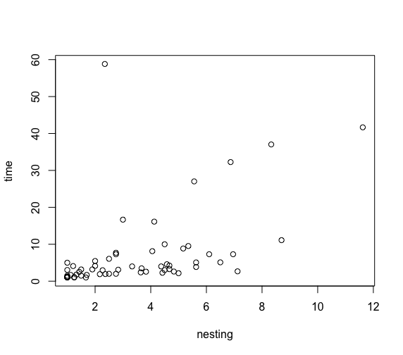
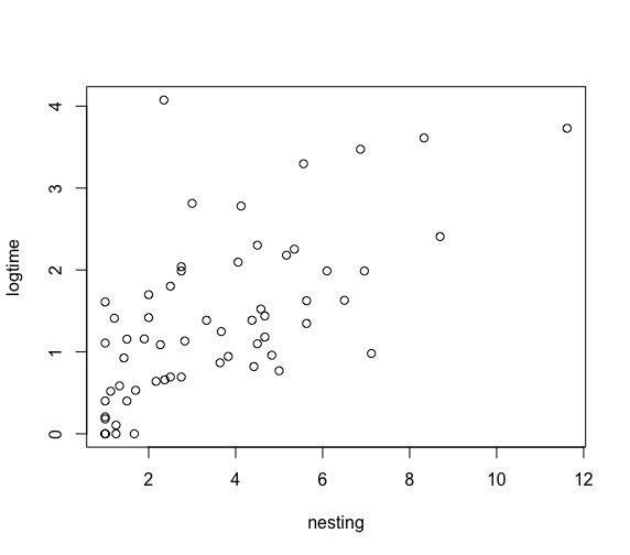
どうやら、timeは対数logtimeを取ったほうがよいとのこと。
> logtime=log(time)
> plot(nesting,logtime)
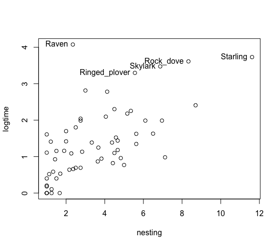
絶滅期間の対数値が3を超えるものの鳥名を記載する。
> out = (logtime > 3)
> text(nesting[out], logtime[out], label=species[out], pos = 2)
サイズ(size, 小0か大1)と絶滅期間の関係も散布図で確認、jitterでドットの重なりをずらし、xaxpでX軸メモリ指定。
> plot(jitter(size),logtime,xaxp=c(0,1,1))

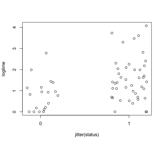
渡り鳥(status, 渡り鳥0か留鳥1)かどうかと、絶滅期間の関係も散布図で確認
> plot(jitter(status),logtime,xaxp=c(0,1,1))
ここで回帰モデルを以下のように設定:
E(log TIMEi|x,θ) = β0 + β1*NESTINGi + β2*SIZEi + β3*STATUSi
まずは、lm()関数を使って、最小二乗法で古典的に分析してみる。
> fit=lm(logtime~nesting+size+status,data=birdextinct,x=TRUE,y=TRUE)
> summary(fit)
Call:
lm(formula = logtime ~ nesting + size + status, data = birdextinct,
x = TRUE, y = TRUE)
Residuals:
Min 1Q Median 3Q Max
-1.8410 -0.2932 -0.0709 0.2165 2.5167
Coefficients:
Estimate Std. Error t value Pr(>|t|)
(Intercept) 0.43087 0.20706 2.081 0.041870 *
nesting 0.26501 0.03679 7.203 1.33e-09 ***
size -0.65220 0.16667 -3.913 0.000242 ***
status 0.50417 0.18263 2.761 0.007712 **
—
Signif. codes: 0 ‘***’ 0.001 ‘**’ 0.01 ‘*’ 0.05 ‘.’ 0.1 ‘ ’ 1
Residual standard error: 0.6524 on 58 degrees of freedom
Multiple R-squared: 0.5982, Adjusted R-squared: 0.5775
F-statistic: 28.79 on 3 and 58 DF, p-value: 1.577e-11
lm()関数で、x=TRUE, y=TRUEとしたことで、デザイン行列と反応のベクトルはオブジェクトfitの要素となる。
回帰モデルにおける「デザイン行列」の定義については、以下のサイトを参照>
http://www012.upp.so-net.ne.jp/doi/biostat/CT39/design_mtx.pdf
> fit$x
(Intercept) nesting size status
1 1 1.000 0 1
2 1 2.000 0 1
3 1 1.210 0 1
4 1 1.125 0 1
5 1 5.167 0 1
6 1 1.000 0 0
7 1 2.750 0 1
8 1 5.630 0 1
9 1 3.000 0 1
10 1 4.670 0 0
11 1 4.056 0 1
12 1 1.000 0 1
13 1 6.960 0 0
14 1 1.670 0 0
15 1 5.560 0 1
16 1 2.830 0 0
17 1 4.375 0 0
18 1 4.125 0 0
19 1 3.670 0 1
20 1 8.330 0 1
21 1 2.750 0 1
22 1 1.430 0 0
23 1 2.000 0 1
24 1 2.750 0 1
25 1 4.500 0 1
26 1 7.120 0 1
27 1 4.580 0 1
28 1 2.350 0 1
29 1 6.870 1 1
30 1 3.830 1 0
31 1 5.000 1 0
32 1 1.250 1 0
33 1 2.270 1 1
34 1 5.350 1 1
35 1 8.700 1 1
36 1 6.100 1 1
37 1 3.330 1 1
38 1 3.640 1 1
39 1 4.830 1 0
40 1 4.670 1 1
41 1 1.700 1 1
42 1 1.330 1 1
43 1 1.000 1 0
44 1 1.900 1 0
45 1 4.420 1 0
46 1 1.250 1 0
47 1 1.000 1 0
48 1 1.000 1 1
49 1 1.000 1 0
50 1 2.500 1 1
51 1 1.500 1 1
52 1 2.500 1 1
53 1 5.630 1 1
54 1 2.370 1 1
55 1 1.500 1 1
56 1 1.000 1 1
57 1 6.500 1 1
58 1 4.500 1 1
59 1 2.170 1 1
60 1 11.620 1 1
61 1 1.000 1 0
62 1 1.000 1 1
attr(,”assign”)
[1] 0 1 2 3
> fit$y
1 2 3 4 5 6 7 8
1.1085626 1.6981811 1.4104990 0.5193889 2.1804175 0.4007875 2.0401808 1.3470336
9 10 11 12 13 14 15 16
2.8134307 1.4395981 2.0955609 1.6094379 1.9877374 0.0000000 3.2968364 1.1333357
17 18 19 20 21 22 23 24
1.3862944 2.7806189 1.2481811 3.6119174 1.9877374 0.9262411 1.4187616 0.6931472
25 26 27 28 29 30 31 32
2.3025851 0.9809542 1.5232262 4.0745499 3.4737661 0.9442949 0.7701082 0.0000000
33 34 35 36 37 38 39 40
1.0875513 2.2538149 2.4079356 1.9877374 1.3862944 0.8675206 0.9597333 1.1808065
41 42 43 44 45 46 47 48
0.5312163 0.5850050 0.1806535 1.1584523 0.8211005 0.1052605 0.0000000 0.0000000
49 50 51 52 53 54 55 56
0.2070142 1.8018748 1.1553076 0.6931472 1.6245235 0.6595904 0.4007875 0.0000000
57 58 59 60 61 62
1.6296326 1.0996118 0.6408007 3.7297094 0.0000000 0.0000000
blinreg()関数を使って、事後結合分布から標本を求める
ーーーーーーーーーーーーーーー
Usage
blinreg(y,X,m,prior=NULL)
Arguments
y
vector of responses
X
design matrix
m
number of simulations desired
prior
list with components c0 and beta0 of Zellner’s g prior
ーーーーーーーーーーーーーーー
> theta.sample=blinreg(fit$y,fit$x,5000)
分散σ^2を逆ガンマ関数((n-k)/2, S/2)からrigamma()関数で抽出する。
> fit$df
[1] 58
> fit$df.residual
[1] 58
> S <- sum(fit$residual^2)
> shape <- fit$df.residual/2; rate <- S/2
> sigma2 <- rigamma(1, shape, rate)
fir$dfは、標本の自由度で、サンプル数62から、変数の個数+1=4を減じた58
次に回帰係数のベクトルβを分散共分散行列Vβσ^2の多変量正規密度からシミュレーションする。
> MSE <- sum(fit$residuals^2)/fit$df.residual
> vbeta <- vcov(fit)/MSE
> beta <- rmnorm(1, mean = fit$coef, varcov = vbeta * sigma2)
回帰係数β1、β2、β3とσをシミュレーションした事後標本のヒストグラムを作成する。
> par(mfrow=c(2,2))
> hist(theta.sample$beta[,2],main=”NESTING”,
+ xlab=expression(beta[1]))
> hist(theta.sample$beta[,3],main=”SIZE”,
+ xlab=expression(beta[2]))
> hist(theta.sample$beta[,4],main=”STATUS”,
+ xlab=expression(beta[3]))
> hist(theta.sample$sigma,main=”ERROR SD”,
+ xlab=expression(sigma))
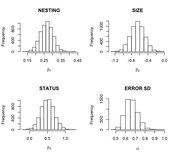
パラメータ毎にシミュレーション標本の5%, 50%, 95%分位点を計算して要約する。
> apply(theta.sample$beta,2,quantile,c(.05,.5,.95))
X(Intercept) Xnesting Xsize Xstatus
5% 0.08500055 0.2026461 -0.9294869 0.2041396
50% 0.42869089 0.2655897 -0.6539865 0.5050282
95% 0.76914027 0.3260018 -0.3786164 0.8198167
>
> quantile(theta.sample$sigma,c(.05,.5,.95))
5% 50% 95%
0.5657864 0.6568641 0.7726691
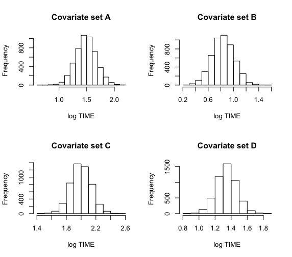
次に、サイズとStatusの異なる組み合わせごとに、4組のNestingと絶滅期間の対数の平均を推定する。
これらの集合をX1にまとめる。
blinregexpected()関数は、共変量の各集合について、その期待反応のシミュレーション出力を行う。
表9.1は間違っているのでは。>小、大、小、大:渡り鳥、渡り鳥、留鳥、留鳥の順。
> cov1=c(1,4,0,0)
> cov2=c(1,4,1,0)
> cov3=c(1,4,0,1)
> cov4=c(1,4,1,1)
> X1=rbind(cov1,cov2,cov3,cov4)
> mean.draws=blinregexpected(X1,theta.sample)
> c.labels=c(“A”,”B”,”C”,”D”)
>
> par(mfrow=c(2,2))
> for (j in 1:4)
+ hist(mean.draws[,j],
+ main=paste(“Covariate set”,c.labels[j]),xlab=”log TIME”)
次にblinregpred()関数は、ある変量xiが与えられたときの回帰モデルの将来の反応値yをシミュレーションした標本を生成する。
> cov1=c(1,4,0,0)
> cov2=c(1,4,1,0)
> cov3=c(1,4,0,1)
> cov4=c(1,4,1,1)
> X1=rbind(cov1,cov2,cov3,cov4)
> pred.draws=blinregpred(X1,theta.sample)
>
> c.labels=c(“A”,”B”,”C”,”D”)
>
> par(mfrow=c(2,2))
> for (j in 1:4)
+ hist(pred.draws[,j],
+ main=paste(“Covariate set”,c.labels[j]),xlab=”log TIME”)
>
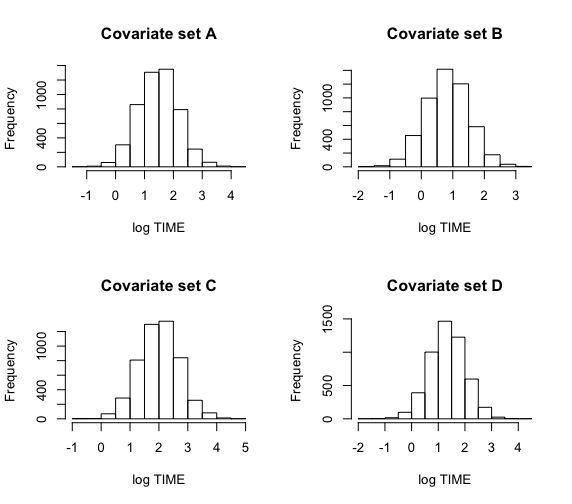
上記2つのグラフの違いは、平均値の予測分布と、反応値の予測分布。当然、後者のほうが広い分布を示す。
最後にモデルが観測値と矛盾していないか調べてみる。
観測値のxiをbinregpred()関数に与えて、y1の5%-95%分位点をシミュレーションして、さらに観測値yiを重ねる。
> pred.draws=blinregpred(fit$x,theta.sample)
> pred.sum=apply(pred.draws,2,quantile,c(.05,.95))
> par(mfrow=c(1,1))
> ind=1:length(logtime)
> if (.Platform$OS.type == “unix”) x11() else windows()
> matplot(rbind(ind,ind),pred.sum,type=”l”,lty=1,col=1,
+ xlab=”INDEX”,ylab=”log TIME”)
> points(ind,logtime,pch=19)
> out=(logtime>pred.sum[2,])
> text(ind[out], logtime[out], label=species[out], pos = 4)
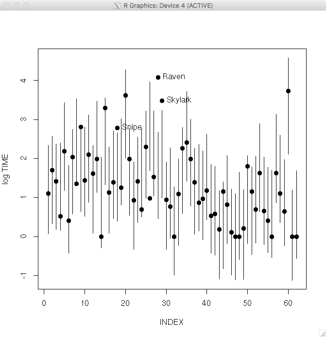
外れ値として、snipe, raven, skylarkが同定された。
もう一つの外れ値の同定には、bayesresiduals()関数を使用する。lm()関数で当てはめたオブジェクトfitとシミュレーションした標本行列theta.sampleとカットオフk=2を与える。事後分布における外れ値の確率を算出する。
> prob.out=bayesresiduals(fit,theta.sample,2)
> par(mfrow=c(1,1))
> plot(nesting,prob.out)
> out = (prob.out > 0.35)
> text(nesting[out], prob.out[out], label=species[out], pos = 4)
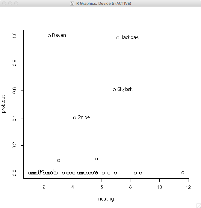
再び、外れ値として、snipe, raven, skylarkに加えてJackdawが同定された。